Chapter 37 Spatially Continuous Data IV
NOTE: The source files for this book are available with companion package {isdas}. The source files are in Rmarkdown format and packed as templates. These files allow you execute code within the notebook, so that you can work interactively with the notes.
37.1 Learning objectives
In the previous practice you were introduced to the concept of variographic analysis for fields/spatially continuous data. In this practice, we will learn:
- How to use residual spatial pattern to estimate prediction errors.
- Kriging: a method for optimal predictions.
37.2 Suggested reading
- Bailey TC and Gatrell AC (1995) Interactive Spatial Data Analysis, Chapters 5 and 6. Longman: Essex.
- Bivand RS, Pebesma E, and Gomez-Rubio V (2008) Applied Spatial Data Analysis with R, Chapter 8. Springer: New York.
- Brunsdon C and Comber L (2015) An Introduction to R for Spatial Analysis and Mapping, Chapter 6, Sections 6.7 and 6.8. Sage: Los Angeles.
- Isaaks EH and Srivastava RM (1989) An Introduction to Applied Geostatistics, Chapter 12. Oxford University Press: Oxford.
- O’Sullivan D and Unwin D (2010) Geographic Information Analysis, 2nd Edition, Chapters 9 and 10. John Wiley & Sons: New Jersey.
37.3 Preliminaries
As usual, remember to begin work with a new session of R. At least, remembert to clear the working space to make sure that you do not have extraneous items there when you begin your work. The command in R to clear the workspace is rm (for “remove”), followed by a list of items to be removed. To clear the workspace from all objects, do the following:
Note that ls() lists all objects currently on the workspace.
Load the libraries you will use in this activity:
Begin by loading the data file:
You can verify the contents of the dataframe:
##       ID                  X               Y               V
##  Length:470         Min.   :  8.0   Min.   :  8.0   Min.   :   0.0
##  Class :character   1st Qu.: 51.0   1st Qu.: 80.0   1st Qu.: 182.0
##  Mode  :character   Median : 89.0   Median :139.5   Median : 425.2
##                     Mean   :111.1   Mean   :141.3   Mean   : 435.4
##                     3rd Qu.:170.0   3rd Qu.:208.0   3rd Qu.: 644.4
##                     Max.   :251.0   Max.   :291.0   Max.   :1528.1
##
##        U           T
##  Min.   :   0.00   1: 45
##  1st Qu.:  83.95   2:425
##  Median : 335.00
##  Mean   : 613.27
##  3rd Qu.: 883.20
##  Max.   :5190.10
##  NA's   :195
37.4 Using residual spatial pattern to estimate prediction errors
Previously, in Chapter @ref{spatially-continuous-data-ii} we discussed how to interpolate a field using trend surface analysis; we also saw how that method may lead to residuals that are not spatially independent.
The implication of non-random residuals is that there is systematic residual pattern that the model did not capture; This, in turn, means that there is at least some information that can still be extracted from the residuals. Again, we will use the case of Walker Lake to explore one way to do this.
As before, we first calculate the polynomial terms of the coordinates to fit a trend surface to the data:
Walker_Lake <- mutate(Walker_Lake,
                      X3 = X^3, X2Y = X^2 * Y, X2 = X^2,
                      XY = X * Y,
                      Y2 = Y^2, XY2 = X * Y^2, Y3 = Y^3)
Given the polynomial expansion, we can proceed to estimate the following cubic trend surface model, which we already know provided the best fit to the data:
WL.trend3 <- lm(formula = V ~ X3 + X2Y + X2 + X + XY + Y + Y2 + XY2 + Y3,
                data = Walker_Lake)
summary(WL.trend3)
##
## Call:
## lm(formula = V ~ X3 + X2Y + X2 + X + XY + Y + Y2 + XY2 + Y3,
## data = Walker_Lake)
##
## Residuals:
## Min 1Q Median 3Q Max
## -564.19 -197.41 7.91 194.25 929.72
##
## Coefficients:
## Estimate Std. Error t value Pr(>|t|)
## (Intercept) -8.620e+00 1.227e+02 -0.070 0.944035
## X3 1.533e-04 4.806e-05 3.190 0.001522 **
## X2Y 6.139e-05 3.909e-05 1.570 0.117000
## X2 -6.651e-02 1.838e-02 -3.618 0.000330 ***
## X 9.172e+00 2.386e+00 3.844 0.000138 ***
## XY -4.420e-02 1.430e-02 -3.092 0.002110 **
## Y 4.794e+00 2.040e+00 2.350 0.019220 *
## Y2 -1.806e-03 1.327e-02 -0.136 0.891822
## XY2 7.679e-05 2.956e-05 2.598 0.009669 **
## Y3 -4.170e-05 2.819e-05 -1.479 0.139759
## ---
## Signif. codes: 0 '***' 0.001 '**' 0.01 '*' 0.05 '.' 0.1 ' ' 1
##
## Residual standard error: 276.7 on 460 degrees of freedom
## Multiple R-squared: 0.1719, Adjusted R-squared: 0.1557
## F-statistic: 10.61 on 9 and 460 DF, p-value: 5.381e-15We can next visualize the residuals which, as you can see, do not appear to be random
plot_ly(x = ~Walker_Lake$X,
        y = ~Walker_Lake$Y,
        z = ~WL.trend3$residuals,
        color = ~WL.trend3$residuals < 0,
        colors = c("blue", "red"),
        type = "scatter3d")
## No scatter3d mode specifed:
## Setting the mode to markers
## Read more about this attribute -> https://plotly.com/r/reference/#scatter-modeNow we will create an interpolation grid:
# The function `sequence()` create a sequence of values from - to
# using by as the step increment. In this case, we generate a grid
# with points that are 2.5 m apart.
X.p <- seq(from = 0.1, to = 255.1, by = 2.5)
Y.p <- seq(from = 0.1, to = 295.1, by = 2.5)
df.p <- expand.grid(X = X.p, Y = Y.p)
WE can add the polynomial terms to this grid. Since our trend surface model was estimated using the cubic polynomial, we add those terms to the dataframe:
df.p <- mutate(df.p, X3 = X^3, X2Y = X^2 * Y, X2 = X^2,
               XY = X * Y,
               Y2 = Y^2, XY2 = X * Y^2, Y3 = Y^3)
The interpolated cubic surface is obtained by using the model and the interpolation grid as newdata:
# The function `predict()` is used to make predictions given a model
# and a possibly new dataset, different from the one used for estimation
# of the model.
WL.preds3 <- predict(WL.trend3,
                     newdata = df.p,
                     se.fit = TRUE,
                     interval = "prediction",
                     level = 0.95)
The surface is converted into a matrix for 3D plotting:
And plot:
WL.plot3 <- plot_ly(x = ~X.p,
                    y = ~Y.p,
                    z = ~z.p3,
                    type = "surface",
                    colors = "YlOrRd") |>
  layout(scene = list(aspectmode = "manual",
                      aspectratio = list(x = 1,
                                         y = 1,

                                         z = 1)))
WL.plot3
The trend surface provides a smooth estimate of the field. However, it is not sufficient to capture all systematic variation, and fails to produce random residuals.
A possible way of enhancing this approach to interpolation is to exploit the information that remains in the residuals, for instance by the use of \(k\)-point means.
We can illustrate this as follows. To interpolate the residuals, we first need the set of target points (the points for the interpolation), as well as the source (the observations):
# We will use the prediction grid we used above to interpolate the residuals
target_xy = expand.grid(x = X.p,
                        y = Y.p) |>
  st_as_sf(coords = c("x", "y"))

# Convert the `Walker_Lake` dataframe to a simple features object using as follows:
Walker_Lake.sf <- Walker_Lake |>
  st_as_sf(coords = c("X", "Y"))

# Append the residuals to the table
Walker_Lake.sf$residuals <- WL.trend3$residuals
It is possible now to use the kpointmean function to interpolate the residuals, for instance using \(k=5\) neighbors:
## projected pointsGiven the interpolated residuals, we can join them to the cubic trend surface, as follows:
z.p3 <- matrix(data = WL.preds3$fit[,1] + kpoint.5$z,
               nrow = length(Y.p),
               ncol = length(X.p),
               byrow = TRUE)
This is now the interpolated field that combines the trend surface and the estimated residuals:
WL.plot3 <- plot_ly(x = ~X.p,
                    y = ~Y.p,
                    z = ~z.p3,
                    type = "surface",
                    colors = "YlOrRd") |>
  layout(scene = list(aspectmode = "manual",
                      aspectratio = list(x = 1,
                                         y = 1,
                                         z = 1)))
WL.plot3
Of all the approaches that we have seen so far, this is the first that provides a genuine estimate of the following: \[ \hat{z}_p + \hat{\epsilon}_p \]
With trend surface analysis providing a smooth estimator of the underlying field: \[ \hat{z}_p = f(x_p, y_p) \]
And \(k\)-point means providing an estimator of: \[ \hat{\epsilon}_p \]
A question is how to decide the number of neighbors to use in the calculation of the \(k\)-point means. As previously discussed, \(k\)=1 becomes identical to Voronoi polygons, and \(k = n\) becomes the global mean.
A second question concerns the way the average is calculated. As variographic analysis demonstrates, it is possible to estimate the way in which spatial dependence weakens with distance. Why should more distant points be weighted equally? The answer is, there is no reason why they should, and in fact, variographic analysis elegantly solves this, as well the question of how many points to use: all of them, with varying weights.
Next, we will introduce kriging, a method for optimal prediction that is based on the use of variographic analysis.
37.5 Kriging: a method for optimal prediction.
To introduce the method known as kriging, we will begin by positing a situation as follows:
\[ \hat{z}_p + \hat{\epsilon}_p = \hat{f}(x_p, y_p) + \hat{\epsilon}_p \]
where \(\hat{f}(x_p, y_p)\) is a smooth estimator of an underlying field.
We aim to predict \(\hat{\epsilon}_p\) based on the observed residuals. We use an expression similar to the one used for IDW and \(k\)-point means in Chapter @ref{spatially-continuous-data-i} (we will use \(\lambda\) for the weights to avoid confusing the the weights in variographic analysis):
\[ \hat{\epsilon}_p = \sum_{i=1}^n {\lambda_{pi}\epsilon_i} \]
That is, \(\hat{\epsilon}_p\) is a linear combination of the prediction residuals from the trend: \[ \epsilon_i = z_i - \hat{f}(x_i, y_i) \]
It is possible to define the following expected mean squared error, or prediction variance: \[ \sigma_{\epsilon}^2 = E[(\hat{\epsilon}_p - \epsilon_i)^2] \]
The prediction variance measures how close, on average, the prediction error is to the residuals.
The prediction variance can be decomposed as follows: \[ \sigma_{\epsilon}^2 = E[\hat{\epsilon}_p] + E[\epsilon_i] - 2E[\hat{\epsilon_i\epsilon}_p] \]
It turns out (we will not show the detailed derivation, but it can be consulted here), that the expression for the prediction variance depends on the weights: \[ \sigma_{\epsilon}^2 = \sum_{i=1}^n \sum_{j=1}^n{\lambda_{ip}\lambda_{jp}C_{ij}} + \sigma^2 + 2\sum_{i=1}^{n}{\lambda_{ip}C_{ip}} \] where \(C_{ij}\) is the autocovariance between observations at \(i\) and \(j\), and \(C_{ip}\) is the autocovariance between the observation at \(i\) and prediction location \(p\).
Fortunately for us, the semivariogram and the autocovariance is straightforward: \[ C_{z}(h) =\sigma^2 - \hat{\gamma}_{z}(h) \]
This means that, given the distance \(h\) between \(i\) and \(j\), and \(i\) and \(p\), we can use a semivariogram to obtain the autocovariances needed to calculate the prediction variance. We are still missing, however, the weights \(\lambda\), which are not known a priori.
These weights can be obtained if we use the following rules:
The expectation of the prediction errors is zero (unbiassedness) Find the weights \(lambda\) that minimize the prediction variance (optimal estimator).
This makes sense, since we would like our predictions to be unbiased (i.e., accurate) and as precise as possible, that is, to have the smallest variance (recall the discussion about accuracy and precision in Chapter @ref{spatially-continuous-data-iii}).
Again, solving the minimization problem is beyond the scope of our presentation, but it suffices to say that the result is as follows:
\[ \mathbf{\lambda}_p = \mathbf{C}^{-1}\mathit{c}_{p} \]
where \(\mathbf{C}\) is the covariance matrix, and \(\mathit{c}_{p}\) is the covariance vector for location \(p\).
In summary, kriging is a method to optimally estimate the value of a variable at \(p\) as a weighted sum of the observations of the same variable at locations \(i\). This method is known to have the properties of Best (in the sense that it minimizes the variance) Linear (because predictions are a linear combination of weights) Unbiased (since the estimators of the prediction errors are zero) Predictor, or BLUP.
Kriging is implemented in the package gstat as follows.
To put kriging to work we must first conduct variographic analysis of the residuals. The function variogram uses as an argument a simple features object that we can create as follows:
Walker_Lake.sf <- Walker_Lake |>
  st_as_sf(coords = c("X", "Y"),
           # Remove set to false to retain the X and Y coordinates
           # in the dataframe after they are converted to simple features
           remove = FALSE)
The variogram of the residuals can be obtained by specifying a trend surface in the formula:
variogram_v <- variogram(V ~ X3 + X2Y + X2 + X + XY + Y + Y2 + XY2 + Y3,
                         data = Walker_Lake.sf)

# Plot
ggplot(data = variogram_v,
       aes(x = dist,
           y = gamma)) +
  geom_point() +
  geom_text(aes(label = np),
            # Nudge the labels away from the points
            nudge_y = -1500) +
  xlab("Distance") +
  ylab("Semivariance")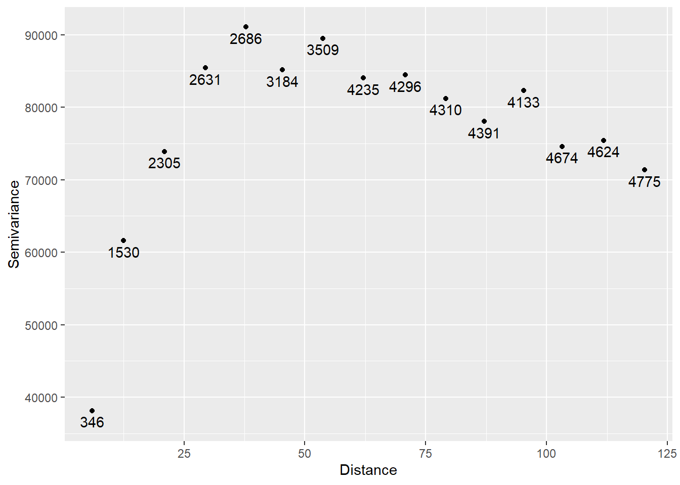
You can verify that the semivariogram above corresponds to the residuals by repeating the analysis directly on the residuals. First join the residuals to the SpatialPointsDataFrame:
And then calculate the semivariogram and plot:
variogram_e <- variogram(e ~ 1,
                         data = Walker_Lake.sf)

# Plot
ggplot(data = variogram_e,
       aes(x = dist,
           y = gamma)) +
  geom_point() +
  geom_text(aes(label = np),
            nudge_y = -1500) +
  xlab("Distance") +
  ylab("Semivariance")
The empirical semivariogram is used to estimate a semivariogram function:
##   model   psill    range
## 1   Nug     0.0 0.000000
## 2   Exp 85554.4 9.910429
The variogram function plots as follows:
gamma.t <- variogramLine(variogram_v.t, maxdist = 130)

# Plot
ggplot(data = variogram_v,
       aes(x = dist,
           y = gamma)) +
  geom_point(size = 3) +
  geom_line(data = gamma.t,
            aes(x = dist,
                y = gamma)) +
  xlab("Distance") +
  ylab("Semivariance")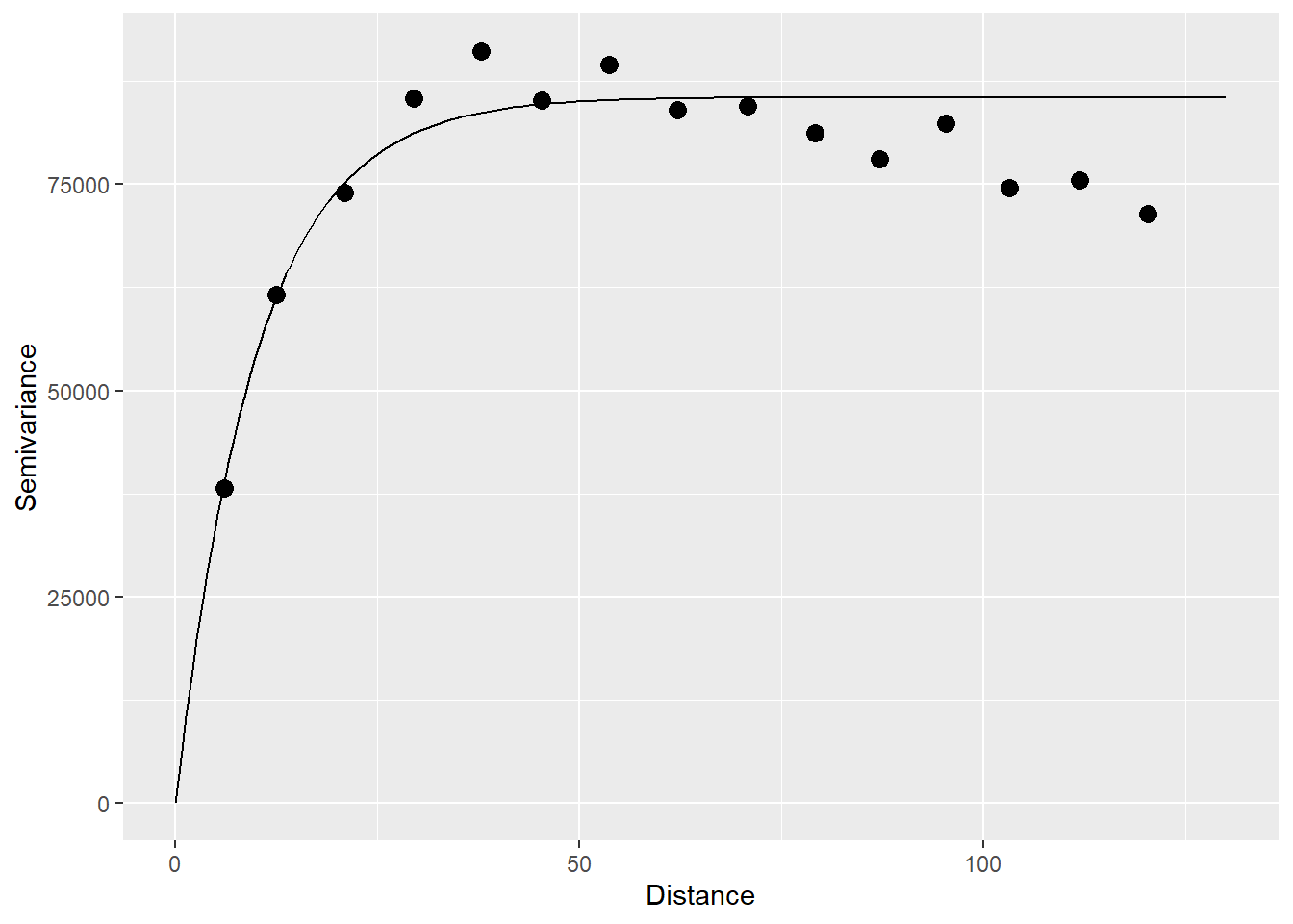
We will convert the prediction grid to a simple features object:
Then, we can krige the field as follows (ensure that packages sf and stars are installed):
V.kriged <- krige(V ~ X3 + X2Y + X2 + X + XY + Y + Y2 + XY2 + Y3,
                  Walker_Lake.sf,
                  df.sf,
                  variogram_v.t)
## [using universal kriging]Extract the predictions and prediction variance from the object V.kriged:
V.km <- matrix(data = V.kriged$var1.pred,
               nrow = 119,
               ncol = 103,
               byrow = TRUE)
V.sm <- matrix(data = V.kriged$var1.var,
               nrow = 119,
               ncol = 103,
               byrow = TRUE)
We can now plot the interpolated field:
V.km.plot <- plot_ly(x = ~X.p,
                     y = ~Y.p,
                     z = ~V.km,
                     type = "surface",
                     colors = "YlOrRd") |>
  layout(scene = list(aspectmode = "manual",
                      aspectratio = list(x = 1,
                                         y = 1,
                                         z = 1)))
V.km.plot
Also, we can plot the kriging standard errors (the square root of the prediction variance). This gives an estimate of the uncertainty in the predictions:
V.sm.plot <- plot_ly(x = ~X.p,
                     y = ~Y.p,
                     z = ~sqrt(V.sm),
                     type = "surface",
                     colors = "YlOrRd") |>
  layout(scene = list(aspectmode = "manual",
                      aspectratio = list(x = 1,
                                         y = 1,
                                         z = 1)))
V.sm.plot
Where are predictions more/less precise?