Chapter 22 Activity 10: Area Data II
NOTE: The source files for this book are available with companion package {isdas}. The source files are in Rmarkdown format and packed as templates. These files allow you execute code within the notebook, so that you can work interactively with the notes.
22.1 Practice questions
Answer the following questions:
- List and describe two criteria to define proximity in area data analysis.
- What is a spatial weights matrix?
- Why do spatial weight matrices have zeros in the main diagonal?
- How is a spatial weights matrix row-standardized?
- Write the spatial weights matrices for the sample systems in Figures @ref{fig:simple-areal-system-i} and @ref{fig:simple-areal-system-ii}. Explain the criteria used to do so.
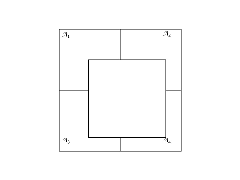
FIGURE 22.1: Sample areal system 1
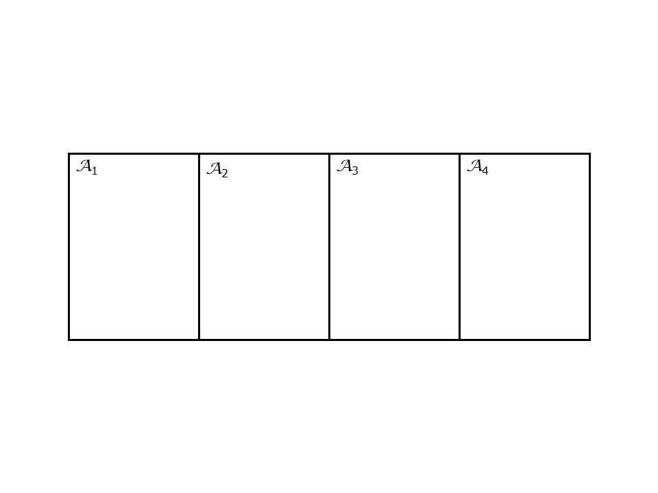
FIGURE 22.2: Sample areal system 2
22.2 Learning objectives
In this activity, you will:
- Create spatial weights matrices.
- Calculate the spatial moving average of a variable.
- Create scatterplots of a variable and its spatial moving average.
- Think about ways to decide whether a landscape is random when working with area data.
22.3 Suggested reading
O’Sullivan D and Unwin D (2010) Geographic Information Analysis, 2nd Edition, Chapter 7. John Wiley & Sons: New Jersey.
22.4 Preliminaries
Remember to restart your R session or at least clear all extraneous objects from the workspace with rm (for “remove”), followed by a list of items to be removed. To clear the workspace from all objects, do the following:
Note that ls() lists all objects currently on the workspace.
Load the libraries you will use in this activity.
In addition to tidyverse, you will need sf, a package that implements simple features in R (you can learn about sf here) and spdep, a package that implements several spatial statistical methods (you can learn more about it here):
In the practice that preceded this activity, you learned about the area data and visualization techniques for area data.
Begin by loading the data that you will use in this activity:
This is a sf object with census tracts and selected demographic variables for the Hamilton CMA in Canada.
You can obtain new (calculated) variables as follows. For instance, to obtain the proportion of residents who are between 20 and 34 years old, and between 35 and 49:
Hamilton_CT <- Hamilton_CT |>
  mutate(Prop20to34 = (AGE_20_TO_24 + AGE_25_TO_29 + AGE_30_TO_34)/POPULATION,
         Prop35to49 = (AGE_35_TO_39 + AGE_40_TO_44 + AGE_45_TO_49)/POPULATION)
You are now ready for the next activity.
22.5 Activity
NOTE: Activities include technical “how to” tasks/questions. Usually, these ask you to practice using the software to organize data, create plots, and so on in support of analysis and interpretation. The second type of questions ask you to activate your brainware and to think geographically and statistically.
Activity Part I
Create a spatial weights matrix for the census tracts in the Hamilton CMA. Use adjacency as your criterion for proximity.
Calculate the spatial moving average for the following two variables: 1) proportion of the population who are 20 to 34 years old; and 2) proportion of the population who are 65 and older.
Append the spatial moving averages to your dataframe.
Choose one age group and create a scatterplot of the proportion of population in that group versus its spatial moving average. (Hint: if you create the scatterplot using
ggplot2you can add the 45 degree line by means ofgeom_abline(slope = 1, intercept = 0)).
Activity Part II
Show your scatterplot of the population versus its spatial moving average to a fellow student. Discuss what you believe is the meaning of the 45 degree line in this plot.
Create a null-landscape by scrambling the values of your variable. For instance, you can use the variable
prop20to34to generate a null landscape as follows:
- Calculate the spatial moving average of your null landscape, and create a scatterplot just like you did for your variable. How is this scatterplot different from the plot created in Question 4?