Chapter 29 Area Data VI
NOTE: The source files for this book are available with companion package {isdas}. The source files are in Rmarkdown format and packed as templates. These files allow you execute code within the notebook, so that you can work interactively with the notes.
29.1 Learning Objectives
In the previous chapter, you practiced how to estimate linear regression models in R, learned about the use of Moran’s \(I\) as a diagnostic tool for regression residuals, and learned how the use local spatial statistics to support model-building. In this practice, you will:
- Revisit the notion of autocorrelation as a model diagnostic.
- Remedial action when the residuals are autocorrelated.
- Flexible functional forms and models with spatially-varying coefficients. 3.1 Trend surface analysis. 3.2 The expansion method. 3.3 Geographically weighted regression (GWR).
- Spatial error model (SEM).
29.2 Suggested Readings
- Bailey TC and Gatrell AC (1995) Interactive Spatial Data Analysis, Chapter 7. Longman: Essex.
- Bivand RS, Pebesma E, and Gomez-Rubio V (2008) Applied Spatial Data Analysis with R, Chapter 9. Springer: New York.
- Brunsdon C and Comber L (2015) An Introduction to R for Spatial Analysis and Mapping, Chapter 7. Sage: Los Angeles.
- O’Sullivan D and Unwin D (2010) Geographic Information Analysis, 2nd Edition, Chapter 7. John Wiley & Sons: New Jersey.
29.3 Preliminaries
Remember that it is good practice to begin your work with a new R session. To reduce the risk of errors caused by extraneous items in memory, you should at least clear the working space. The command in R to clear the workspace is rm (for “remove”), followed by a list of items to be removed. To clear the workspace from all objects, do the following:
Note that ls() lists all objects currently on the workspace.
Load the libraries you will use in this activity:
library(isdas)
library(kableExtra)
library(plotly)
library(sf)
library(spatialreg)
library(spdep)
library(spgwr)
library(tidyverse)
Begin by loading the data needed for this chapter:
This is a simple features sf object with the the Dissemination Areas in the Hamilton Census Metropolitan Area, in Canada, and it includes five simulated variables.
29.4 Residual spatial autocorrelation revisited
A key assumption about the residuals of a regression model is that they are random, which means that they cannot have residual systematic pattern. Previously you learned about the use of Moran’s \(I\) coefficient as a diagnostic in regression analysis. The residuals of a model can be mapped and examined for pattern, and Moran’s \(I\) used to test the hypothesis that they are spatially random. When we reject the null hypothesis and conclude that the residuals are not random, this is a symptom of a model that has not been properly specified.
Here, we will focus on two reasons for this that are of interest:
- The functional form is incorrect.
- The model failed to include relevant variables.
We will explore these in turn.
29.4.1 Incorrect Functional Form
As we say in the preceding chapter, linear regression means that the parameters of the model are linear. However, life is not always linear, and an incorrect functional form can lead to residual spatial autocorrelation (McMillen 2003). To illustrate this, we will consider a spatial process as follows: \[ z = f(u,v) = exp(\beta_0)exp(\beta_1u)exp(\beta_2v) \]
where \(u\) and \(v\) are spatial coordinates. This is a non-linear spatial process, since the relationship between the coefficients and the outcome is not linear. We can simulate this process if we use the spatial coordinates of the dissemination areas in our example. The simulation is as follows, with a residual term with a mean of zero and standard deviation of 1. Notice that the residuals are random by design:
# The function `set.seed()` is used to fix the seed for the random number generator. This ensures that the simulation is replicable.
set.seed(10)

# Set the coefficients of the model for the simulations.
b0 = 1
b1 = 2
b2 = 4

# Retrieve the coordinates of the centroids of the dissemination areas.
uv_coords <- st_coordinates(st_centroid(HamiltonDAs))
## Warning: st_centroid assumes attributes are constant over geometries# Add the coordinates of the centroids to the dataframe, but first transform them so that they have a false origin at the minimum values of u and v, and scaled by 100000. Simulate variable z using the coefficients defined above, the transformed coordinates, and add a random component with a mean of zero and standard deviation of one.
HamiltonDAs <- HamiltonDAs |>
mutate(u = (uv_coords[,1] - min(uv_coords[,1]))/100000,
v = (uv_coords[,2] - min(uv_coords[,2]))/100000,
z = exp(b0) * exp(b1 * u) * exp(b2 * v) +
rnorm(n = 297, mean = 0, sd = 1))This is the summary of the simulated variables:
##        u                v                z                   geometry
##  Min.   :0.0000   Min.   :0.0000   Min.   : 3.919   MULTIPOLYGON :297
##  1st Qu.:0.2284   1st Qu.:0.1354   1st Qu.: 7.842   epsg:26917   :  0
##  Median :0.2695   Median :0.1712   Median : 9.370   +proj=utm ...:  0
##  Mean   :0.2724   Mean   :0.1863   Mean   :10.370
##  3rd Qu.:0.3127   3rd Qu.:0.2195   3rd Qu.:11.710
##  Max.   :0.5312   Max.   :0.4079   Max.   :22.809
Suppose that we estimate the model as a linear regression that fails to correctly capture the non-linearity by specifying linear parameters. The model would be as follows:
##
## Call:
## lm(formula = z ~ u + v, data = HamiltonDAs)
##
## Residuals:
##     Min      1Q  Median      3Q     Max
## -2.7267 -0.8591  0.0028  0.8250  3.5826
##
## Coefficients:
##             Estimate Std. Error t value Pr(>|t|)
## (Intercept)  -3.6765     0.3255  -11.29   <2e-16 ***
## u            20.9207     0.8586   24.37   <2e-16 ***
## v            44.8033     0.9305   48.15   <2e-16 ***
## ---
## Signif. codes:  0 '***' 0.001 '**' 0.01 '*' 0.05 '.' 0.1 ' ' 1
##
## Residual standard error: 1.231 on 294 degrees of freedom
## Multiple R-squared:  0.8965, Adjusted R-squared:  0.8958
## F-statistic:  1273 on 2 and 294 DF,  p-value: < 2.2e-16
At first glance, the model gives the impression of a very good fit: all coefficients are significant, and the coefficient of multiple determination \(R^2\) is high. However, at this point it is important to examine the residuals to verify that they are independent. We will add the residuals of this model to the dataframe for visualization:
# Copy the residuals of the model to the dataframe for mapping
HamiltonDAs$model1.e <- model1$residuals
A map of the residuals can help s to examine their spatial pattern (negative residuals are red, positive are blue):
# Create a `plotly` object with the dataframe and plot the the simple features object with colors per the sign of the residuals (negative residuals = FALSE, positive residuals = TRUE)
  plot_ly(HamiltonDAs) |>
    add_sf(color = ~ifelse(model1.e > 0, "Positive", "Negative"), colors = c("red", "dodgerblue4"))
Visual inspection of the spatial distribution of residuals is suggestive. Positive residuals mean that the model underestimates the values of the dependent variable, and negative that the model overestimates the values of the dependent variable. The model systematically underestimates the variable along a north-south band that crosses the center of the region, and overestimates systematically to the east and west. While it is quite clear that there is systematic residual pattern, it is important to support our visual inspection of the residuals by testing for spatial residual autocorrelations.
To do this, we need to create a set of spatial weights:
Once that we have a set of spatial weights, we can proceed to calculate Moran’s \(I\):
##
##  Moran I test under randomisation
##
## data:  HamiltonDAs$model1.e
## weights: HamiltonDAs.w
##
## Moran I statistic standard deviate = 10.373, p-value < 2.2e-16
## alternative hypothesis: greater
## sample estimates:
## Moran I statistic       Expectation          Variance
##       0.350300067      -0.003378378       0.001162633
Notice the very small \(p\)-value: this result means that we can comfortably reject the null hypothesis of spatial randomness; however, what we wish is the opposite, since we want the residuals to be spatially random! Thus, despite the apparent goodness of fit of the model, there is reason to believe something is amiss with the model (since we simulated it, we know that the problem is that the model should not be linear).
The results of testing for autocorrelation indicate an issue with the model, which in this case is an incorrect specification. This is fixed if we use a variable transformation to approximate the underlying non-linear process. We can take the logarithm on both sides of the equation. On the left hand side, we are left with \(log(z)\). On the right hand, the products become a sum, and the logarithms and exponentials cancel each other, to give: \[ log(z) = log\big(exp(\beta_0)exp(\beta_1u)exp(\beta_2v)\big) = log\big(exp(\beta_0)\big) + log\big(exp(\beta_1u)\big) + log\big(exp(\beta_2v)\big) = \beta_0 + \beta_1u + \beta_2v \]
which is now a linear model. This is called a log-transformation. The log-transformed model is estimated as follows:
##
## Call:
## lm(formula = log(z) ~ u + v, data = HamiltonDAs)
##
## Residuals:
##      Min       1Q   Median       3Q      Max
## -0.32033 -0.06456  0.00671  0.07647  0.31233
##
## Coefficients:
##             Estimate Std. Error t value Pr(>|t|)
## (Intercept)  0.96853    0.02864   33.81   <2e-16 ***
## u            2.08863    0.07554   27.65   <2e-16 ***
## v            3.97537    0.08187   48.56   <2e-16 ***
## ---
## Signif. codes:  0 '***' 0.001 '**' 0.01 '*' 0.05 '.' 0.1 ' ' 1
##
## Residual standard error: 0.1083 on 294 degrees of freedom
## Multiple R-squared:  0.9016, Adjusted R-squared:  0.901
## F-statistic:  1348 on 2 and 294 DF,  p-value: < 2.2e-16
This model does not necessarily have a better goodness of fit. However, when we test for spatial autocorrelation:
##
##  Moran I test under randomisation
##
## data:  HamiltonDAs$model2.e
## weights: HamiltonDAs.w
##
## Moran I statistic standard deviate = 0.59638, p-value = 0.2755
## alternative hypothesis: greater
## sample estimates:
## Moran I statistic       Expectation          Variance
##       0.016946454      -0.003378378       0.001161482
Once that the correct functional form has been specified, the model is better at capturing the underlying process (check how the coefficients closely approximate the true coefficients of the model). In addition, we can conclude that the residuals are random, and therefore are now also spatially random: meaning the there is nothing left of the process but white noise.
29.4.2 Omitted Variables
Using the same example, suppose now that the functional form of the model is correctly specified, but a relevant variable is missing:
##
## Call:
## lm(formula = log(z) ~ u, data = HamiltonDAs)
##
## Residuals:
##      Min       1Q   Median       3Q      Max
## -0.78563 -0.19306 -0.05461  0.14453  0.91857
##
## Coefficients:
##             Estimate Std. Error t value Pr(>|t|)
## (Intercept)  1.90764    0.06334  30.118  < 2e-16 ***
## u            1.36012    0.22197   6.127 2.85e-09 ***
## ---
## Signif. codes:  0 '***' 0.001 '**' 0.01 '*' 0.05 '.' 0.1 ' ' 1
##
## Residual standard error: 0.3246 on 295 degrees of freedom
## Multiple R-squared:  0.1129, Adjusted R-squared:  0.1099
## F-statistic: 37.54 on 1 and 295 DF,  p-value: 2.853e-09
As before, we will append the residuals to the dataframes:
We can plot a map of the residuals to examine their spatial pattern (negative residuals are red, positive are blue):
  plot_ly(HamiltonDAs) |>
    add_sf(type = "scatter",
           color = ~ifelse(model3.e > 0,
                           "Positive",
                           "Negative"),
           colors = c("red",
                      "dodgerblue4"))
In this case, the visual inspection makes it clear that there is an issue with residual spatial pattern, and using Moran’s \(I\) we can conclude that the residuals are spatially autocorrelated:
##
##  Moran I test under randomisation
##
## data:  HamiltonDAs$model3.e
## weights: HamiltonDAs.w
##
## Moran I statistic standard deviate = 24.921, p-value < 2.2e-16
## alternative hypothesis: greater
## sample estimates:
## Moran I statistic       Expectation          Variance
##       0.846098172      -0.003378378       0.001161895
As seen above, the model with the full set of relevant variables resolves this problem.
29.5 Remedial Action
When spatial autocorrelation is detected in the residuals, further work is warranted. The preceding examples illustrate two possible solutions to the issue of residual pattern:
- Modifications of the model to approximate the true functional form of the process; and
- Inclusion of relevant variables.
Ideally, we would try to ensure that the model is properly specified. In practice, however, it is not always evident what the functional form of the model should be. The search for an appropriate functional form can be guided by theoretical considerations, empirical findings, and experimentation. With respect to inclusion of relevant variables, it is not always possible to find all the information we desire. This could be because of limited resources, or because some aspects of the process are not known and therefore we do not even know what additional information should be collected.
In these cases, it is a fact that residual spatial autocorrelation is problematic.
Fortunately, a number of approaches have been proposed in the literature that can be used for remedial action.
In the following sections we will review some of them.
29.6 Flexible Functional Forms and Models with Spatially-varying Coefficients
Some models use variable transformations to create more flexible functions, while others use adaptive estimation strategies.
29.6.1 Trend Surface Analysis
Trend surface analysis is a simple way to generate relatively flexible regression models with surfaces that are not necessarily linear. This approach consists of using the coordinates as covariates, and transforming them into polynomials of different orders. Seen this way, linear regression is the analog of a trend surface of first degree: \[ z = f(x,y) = \beta_0 + \beta_1u + \beta_2v \] where again \(u\) and \(v\) are the coordinates.
A figure illustrates how the function above creates a regression plane. To visualize this, we need to create a grid of coordinates for plotting:
# The function `expand.grid()` takes two arguments and creates a dataframe from all the combinations of the values. The function `seq()` creates a vector with values starting at `from`, ending at `to`, with step increments given `by`. Here, we create a grid with values in `u` from -2 to 2 and values in `v` from -2 to 2.
df <- expand.grid(u = seq(from = -2, to = 2, by = 0.2), v = seq(from = -2, to = 2, by = 0.2))
Next, select some values for the coefficients (feel free to experiment with these values):
# Define some coefficients (you can change these values if you wish).
b0 <- 0.5 #0.5
b1 <- 1 #1
b2 <- 2 #2

# Create the regression plane. We did not add a random term here because this plane is the systematic component of the model!
z1 <- b0 + b1 * df$u + b2 * df$v
z1 <- matrix(z1, nrow = 21, ncol = 21)
The plot is as follows:
# Create a `plotly` object and add a surface.
plot_ly(z = ~z1) |>
  add_surface() |>
  # The function `layout()` defines several aspects of the plot, in this case the labels for the ticks on the axes and the axes titles.
  layout(scene = list(xaxis = list(ticktext = c("-2", "0", "2"),
                                   tickvals = c(0, 10, 20)),
                      yaxis = list(ticktext = c("-2", "0", "2"),
                                   tickvals = c(0, 10, 20)),
                      xaxis = list(title = "v"),
                      yaxis = list(title = "u")
                      )
         )
The figure above is a linear trend surface, and we can see that the dependent variable z grows as u and v grow.
Higher order trend surfaces can be defined as well. For example, a trend surface of second degree (or quadratic), would be as follows. Notice how it includes all possible quadratic terms, including the product \(xy\): \[ z = f(x,y) = \beta_0 + \beta_1u^2 + \beta_2u + \beta_3uv + \beta_4v + \beta_5v^2 \]
Use the same grid as above to create now a regression surface. Select some coefficients:
b0 <- 0.5 #0.5
b1 <- 2 #2
b2 <- 1 #1
b3 <- 1 #1
b4 <- 1.5 #1.5
b5 <- 0.5 #2.5
z2 <- b0 + b1 * df$u^2 + b2 * df$u + b3 * df$u * df$v + b4 * df$v + b5 * df$v^2
z2 <- matrix(z2, nrow = 21, ncol = 21)
And the plot is as follows:
plot_ly(z = ~z2) |> add_surface() |>
  layout(scene = list(xaxis = list(ticktext = c("-2", "0", "2"), tickvals = c(0, 10, 20)),
                      yaxis = list(ticktext = c("-2", "0", "2"), tickvals = c(0, 10, 20)),
                      xaxis = list(title = "v"),
                      yaxis = list(title = "u")
                      )
         )
Higher order polynomials (i.e., cubic, quartic, etc.) are possible in principle. Something to keep in mind is that the higher the order of the polynomial, the more flexible the surface, which may lead to the following issues:
- Multicollinearity.
u coordinate in the example:
| u | u^2 | u^3 | u^4 | |
|---|---|---|---|---|
| u | 1.00 | 0.00 | 0.92 | 0.00 |
| u^2 | 0.00 | 1.00 | 0.00 | 0.96 |
| u^3 | 0.92 | 0.00 | 1.00 | 0.00 |
| u^4 | 0.00 | 0.96 | 0.00 | 1.00 |
When two variables are highly collinear, the model has difficulties discriminating their relative contribution to the model. This is manifested by inflated standard errors that may depress the significance of the coefficients, and occasionally by sign reversals.
- Overfitting.
Overfitting is another possible consequence of using a trend surface that is too flexible. This happens when a model fits too well the observations used for calibration, but because of this it may fail to fit well new information.
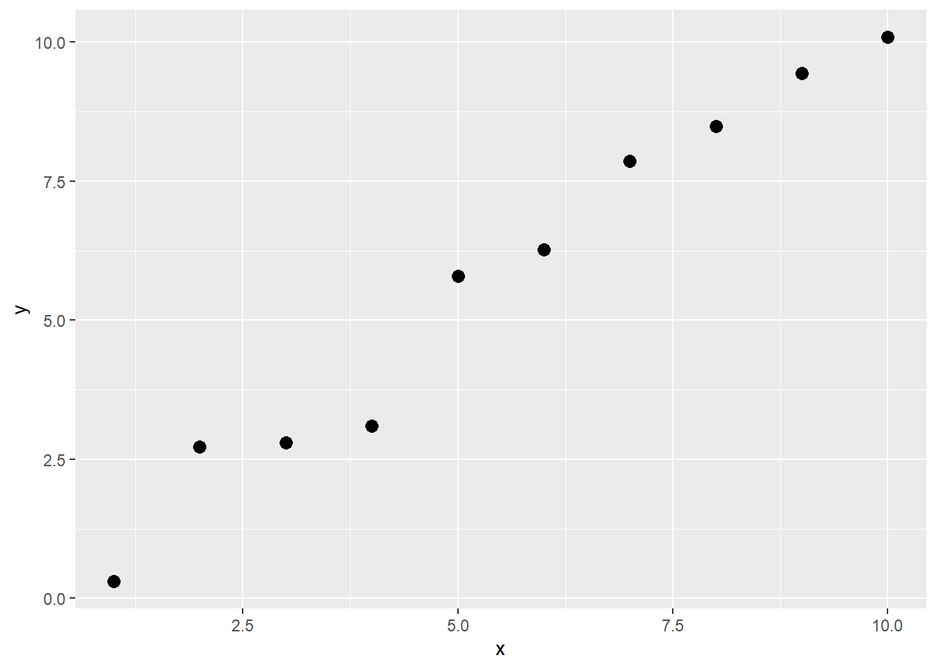
To illustrate overfitting consider a simple example. Below we simulate a simple linear model with \(y_i = x_i + \epsilon_i\) (the random terms are drawn from the uniform distribution). We also simulate new data using the exact same process:
# Dataset for estimation
df.of1 <- data.frame(x = seq(from = 1, to = 10, by = 1))
df.of1 <- mutate(df.of1, y = x + runif(10, -1, 1))
# New data
new_data <- data.frame(x = seq(from = 1, to = 10, by = 0.5))
df.of2 <- mutate(new_data, y = x + runif(nrow(new_data), -1, 1))
This is the scatterplot of the observations in the estimation dataset:
A model with a first order trend (essentially linear regression), does not fit the observations perfectly, but when confronted with new data (plotted as red squares), it predicts them with reasonable accuracy:
mod.of1 <- lm(formula = y ~ x, data = df.of1)
pred1 <- predict(mod.of1, newdata = new_data) #mod.of1$fitted.values
p + geom_abline(slope = mod.of1$coefficients[2], intercept = mod.of1$coefficients[1],
                color = "blue", size = 1) +
  geom_point(data = df.of2, aes(x = x, y = y), shape = 0, color = "red") +
  geom_segment(data = df.of2, aes(xend = x, yend = pred1)) +
  geom_point(size = 3) +
  xlim(c(1, 10))
## Warning: Using `size` aesthetic for lines was deprecated in ggplot2 3.4.0.
## ℹ Please use `linewidth` instead.
## This warning is displayed once every 8 hours.
## Call `lifecycle::last_lifecycle_warnings()` to see where this warning was
## generated.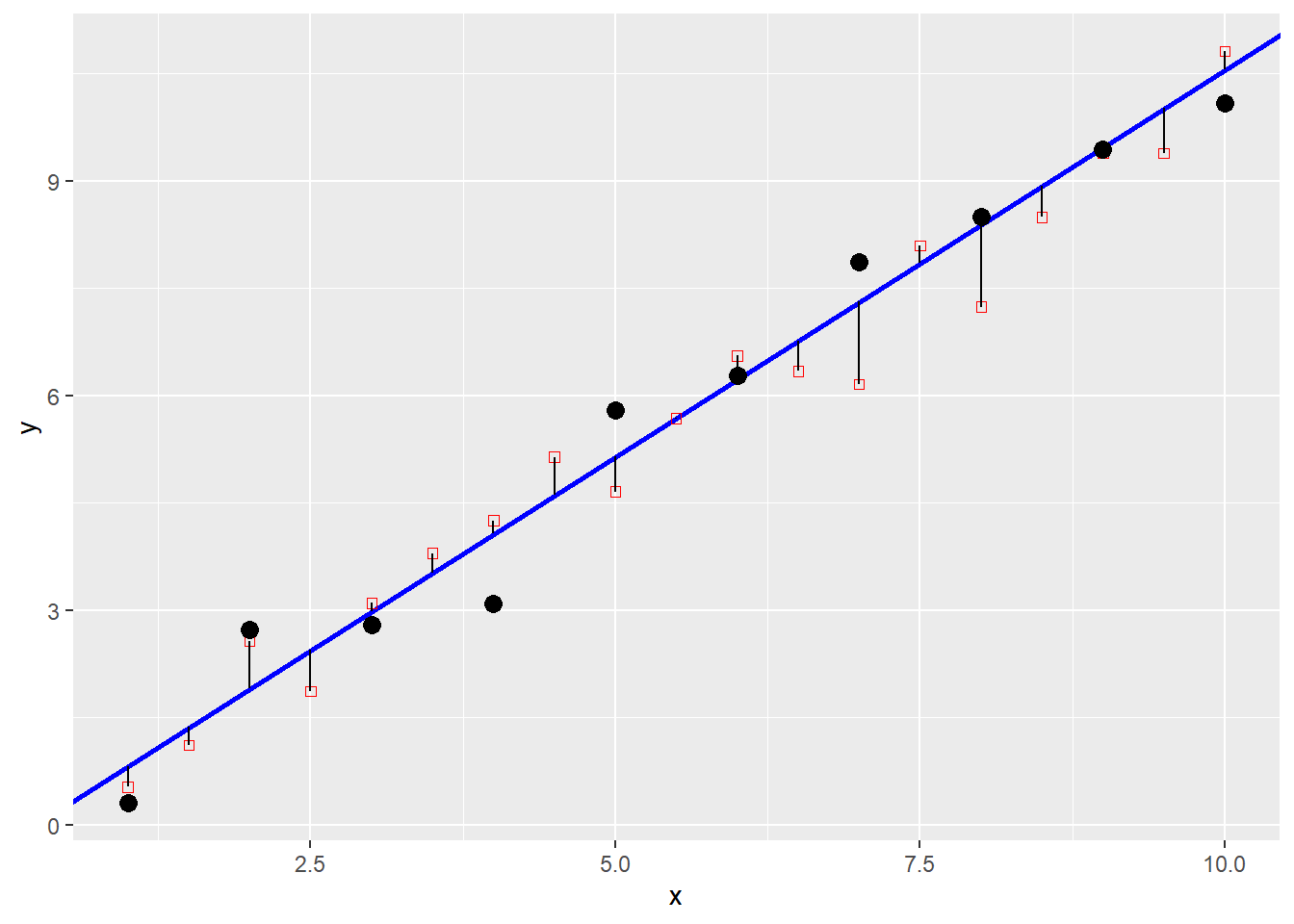
Compare to a polynomial of very high degree (nine in this case). The model is much more flexible, to the extent that it perfectly matches the observations in the estimation dataset. However, this flexibility has a major downside. When the model is confronted with new information, its performance is less satisfactory.
mod.of2 <- lm(formula = y ~ poly(x, degree = 9, raw = TRUE), data = df.of1)
poly.fun <- predict(mod.of2, data.frame(x = seq(1, 10, 0.1)))
pred2 <- predict(mod.of2, newdata = new_data) #mod.of1$fitted.values

p + geom_line(data = data.frame(x = seq(1, 10, 0.1), y = poly.fun),
              aes(x = x, y = y),
              color = "blue", size = 1) +
  geom_point(data = df.of2,
             aes(x = x, y = y),
             shape = 0,
             color = "red") +
  geom_segment(data = df.of2,
               aes(xend = x, yend = pred2)) +
  geom_point(size = 3) +
  xlim(c(1, 10))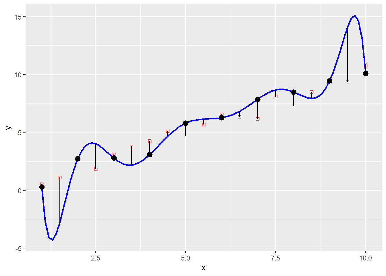
We can compute the root mean square (RMS), for each of the two models. The RMS is a measure of error that is calculated as the square root of the mean of the squared differences between two values (in this case the prediction of the model and the new information). This statistic is a measure of the typical deviation between two sets of values. Given new information, the RMS would tell us the expected size of the error when making a prediction using a given model.
The RMS for model 1 is:
## [1] 0.525595And for model 2:
## [1] 1.681143You will notice how model 2, despite fitting the estimation data better than model 1, typically produces larger errors when new information becomes available.
- Edge effects.
Another consequence of overfitting, is that the resulting functions tend to display extreme behavior when taken outside of their estimation range, where the largest polynomial terms tend to dominate.
The plot below is the same high degree polynomial estimated above, just plotted in a slightly larger range of plus/minus one unit:
poly.fun <- predict(mod.of2, data.frame(x = seq(0, 11, 0.1)))
p +
  geom_line(data = data.frame(x = seq(0, 11, 0.1), y = poly.fun), aes(x = x, y = y),
                color = "blue", size = 1) +
  geom_point(data = df.of2, aes(x = x, y = y), shape = 0, color = "red") +
  geom_segment(data = df.of2, aes(xend = x, yend = pred2)) +
  geom_point(size = 3)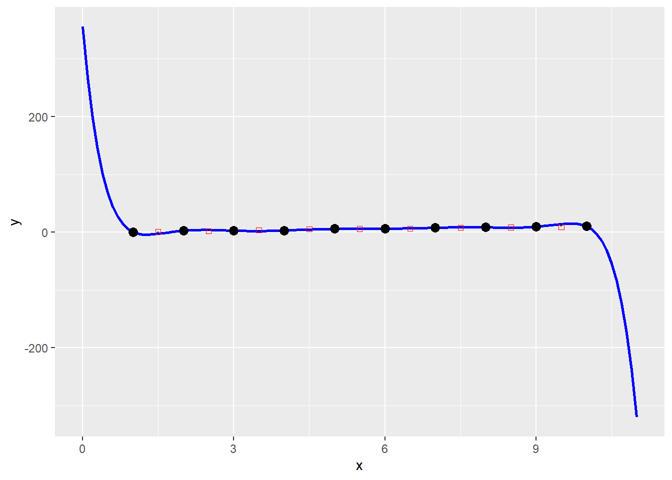
29.6.2 Models with Spatially-varying Coefficients
Another way to generate flexible functional forms is by means of models with spatially varying coefficients. Two approaches are reviewed here.
29.6.2.1 Expansion Method
The expansion method (Casetti, 1972) is an approach to generate models with contextual effects. It follows a philosophy of specifying first a substantive model with variables of interest, and then an expanded model with contextual variables. In geographical analysis, typically the contextual variables are trend surfaces estimated using the coordinates of the observations.
To illustrate this, suppose that there is the following initial model of proportion of donors in a population, with two variables of substantive interest (say, income and education): \[ d_i = \beta_i(u_i,v_i) + \beta_1(u_i,v_i)I_i + \beta_3(u_i,v_i)Ed_i + \epsilon_i \]
Note how the coefficients are now a function of the coordinates at \(i\). Unlike previous models that had global coefficients, the coefficients in this model are allowed to adapt by location.
Unfortunately, it is not possible to estimate one coefficient per location. In this case, there are \(n\times k\) coefficients, which exceeds the size of the sample (\(n\)). It is not possible to retrieve more information from the sample than \(n\) parameters (this is called the incidental parameter problem.)
A possible solution is to specify a function for the coefficients, for instance, by specifying a trend surface for them: \[ \begin{array}{l} \beta_0(u_i, v_i) = \beta_{01} +\beta_{02}u_i + \beta_{03}v_i\\ \beta_1(u_i, v_i) = \beta_{11} +\beta_{12}u_i + \beta_{13}v_i\\ \beta_2(u_i, v_i) = \beta_{21} +\beta_{22}u_i + \beta_{23}v_i \end{array} \] By specifying the coefficients as a function of the coordinates, we allow them to vary by location.
Next, if we substitute these coefficients in the initial model, we arrive at a final expanded model: \[ d_i = \beta_{01} +\beta_{02}u_i + \beta_{03}v_i + \beta_{11}I_i +\beta_{12}u_iI_i + \beta_{13}v_iI_i + \beta_{21}Ed_i +\beta_{22}u_iEd_i + \beta_{23}v_iEd_i + \epsilon_i \]
This model has now nine coefficients, instead of \(n\times 3\), and can be estimated as usual.
It is important to note that since models generated based on the expansion method are based on the use of trend surfaces, similar caveats apply with respect to multicollinearity and overfitting.
29.6.2.2 Geographically Weighted Regression (GWR)
A different strategy to estimate models with spatially-varying coefficients is a semi-parametric approach, called geographically weighted regression (see Brunsdon et al., 1996).
Instead of selecting a functional form for the coefficients as the expansion method does, the functions are left unspecified. The spatial variation of the coefficients results from an estimation strategy that takes subsamples of the data in a systematic way.
If you recall kernel density analysis, a kernel was a way of weighting observations based on their distance from a focal point.
Geographically weighted regression applies a similar concept, with a moving window that visits a focal point and estimates a weighted least squares model at that location. The results of the regression are conventionally applied to the focal point, in such a way that not only the coefficients are localized, but also every other regression diagnostic (e.g., the coefficient of determination, the standard deviation, etc.)
A key aspect of implementing this model is the selection of the kernel bandwidth, that is, the size of the window. If the window is too large, the local models tend towards the global model (estimated using the whole sample). If the window is too small, the model tends to overfit, since in the limit each window will contain only one, or a very small number of observations.
The kernel bandwidth can be selected if we define some loss function that we wish to minimize. A conventional approach (but not the only one), is to minimize a cross-validation score of the following form: \[ CV (\delta) = \sum_{i=1}^n{\big(y_i - \hat{y}_{\neq i}(\delta)\big)^2} \] In this notation, \(\delta\) is the bandwidth, and \(\hat{y}_{\neq i}(\delta)\) is the value of \(y\) predicted by a model with a bandwidth of \(\delta\) after excluding the observation at \(i\). This is called a leave-one-out cross-validation procedure, used to prevent the estimation from shrinking the bandwidth to zero.
GWR is implemented in R in the package spgwr. To estimate models using this approach, the function sel.GWR, which takes as inputs a formula specifying the dependent and independent variables, a SpatialPolygonsDataFrame (or a SpatialPointsDataFrame), and the kernel function (in the example below a Gaussian kernel). Since our data come in the form of simple features, we use as(x, "Spatial") to convert to a Spatial*DataFrame object:
## Bandwidth: 25621.66 CV score: 416.6583
## Bandwidth: 41415.33 CV score: 439.9313
## Bandwidth: 15860.64 CV score: 373.3401
## Bandwidth: 9827.993 CV score: 326.3479
## Bandwidth: 6099.614 CV score: 301.3906
## Bandwidth: 3795.349 CV score: 307.3175
## Bandwidth: 5784.775 CV score: 300.0247
## Bandwidth: 5317.712 CV score: 298.6785
## Bandwidth: 4736.221 CV score: 298.7873
## Bandwidth: 5058.919 CV score: 298.4138
## Bandwidth: 5051.908 CV score: 298.4127
## Bandwidth: 5032.504 CV score: 298.4117
## Bandwidth: 5034.856 CV score: 298.4117
## Bandwidth: 5034.926 CV score: 298.4117
## Bandwidth: 5034.918 CV score: 298.4117
## Bandwidth: 5034.918 CV score: 298.4117
## Bandwidth: 5034.918 CV score: 298.4117
## Bandwidth: 5034.918 CV score: 298.4117
The function gwr estimates the suite of local models given a bandwidth:
model.gwr <- gwr(formula = z ~ u + v,
                 bandwidth = delta,
                 data = as(HamiltonDAs, "Spatial"),
                 gweight = gwr.Gauss)
model.gwr
## Call:
## gwr(formula = z ~ u + v, data = as(HamiltonDAs, "Spatial"), bandwidth = delta,
## gweight = gwr.Gauss)
## Kernel function: gwr.Gauss
## Fixed bandwidth: 5034.918
## Summary of GWR coefficient estimates at data points:
## Min. 1st Qu. Median 3rd Qu. Max. Global
## X.Intercept. -16.8369 -5.8339 -2.0390 -0.6852 2.0016 -3.6765
## u 6.1497 16.5814 19.1775 24.9633 36.8438 20.9207
## v 22.3026 31.5813 36.8539 47.5515 84.3637 44.8033The results are given for each location where a local regression was estimated. We can join these results to our sf dataframe for plotting:
HamiltonDAs$beta0 <- model.gwr$SDF@data$X.Intercept.
HamiltonDAs$beta1 <- model.gwr$SDF@data$u
HamiltonDAs$beta2 <- model.gwr$SDF@data$v
HamiltonDAs$localR2 <- model.gwr$SDF@data$localR2
HamiltonDAs$gwr.e <- model.gwr$SDF@data$gwr.e
The results can be mapped as shown below (try mapping beta1, beta2, localR2, or the residuals gwr.e):
ggplot(data = HamiltonDAs, aes(fill = beta0)) +
  geom_sf(color = "white") +
  scale_fill_distiller(palette = "YlOrRd", trans = "reverse")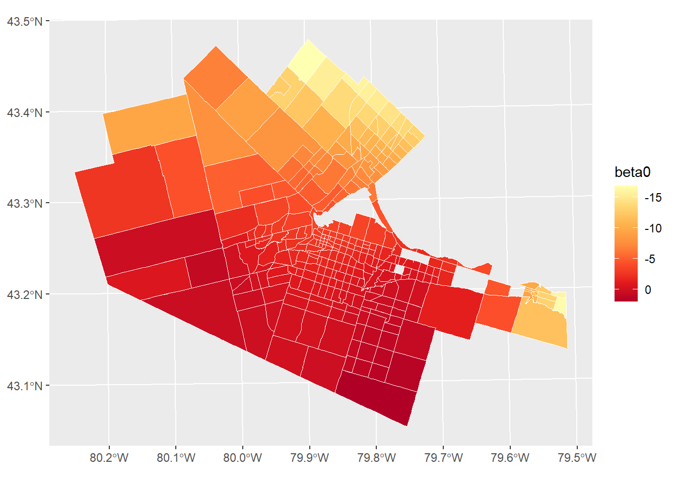
You can verify that the residuals are not spatially autocorrelated:
##
##  Moran I test under randomisation
##
## data:  HamiltonDAs$gwr.e
## weights: HamiltonDAs.w
##
## Moran I statistic standard deviate = 0.016155, p-value = 0.4936
## alternative hypothesis: greater
## sample estimates:
## Moran I statistic       Expectation          Variance
##      -0.002827160      -0.003378378       0.001164184
Some caveats with respect to GWR.
Since estimation requires the selection of a kernel bandwidth, and a kernel bandwidth requires the estimation of many times leave-one-out regressions, GWR can be computationally demanding, especially for large datasets.
GWR has become a very popular method, however, there is conflicting evidence regarding its ability to retrieve a known spatial process (Paez, Farber, and Wheeler 2011). For this reasons, interpretation of the spatially-varying coefficients must be conducted with a grain of salt, although this seems to be less of a concern with larger samples - but at the moment it is not known how large a sample is safe (and larger samples also become computationally more demanding). As well, the estimation method is known to be sensitive to unusual observations (Farber and Páez 2007). At the moment, I recommend that GWR be used for prediction only, and in this respect it seems to perform as well, or even better than alternatives approaches (Paez, Long, and Farber 2008).
29.7 Spatial Error Model (SEM)
A model that can be used to take direct remedial action with respect to residual spatial autocorrelation is the spatial error model.
This model is specified as follows: \[ y_i = \beta_0 + \sum_{j=1}^k{\beta_kx_{ij}} + \epsilon_i \]
However, it is no longer assumed that the residuals \(\epsilon\) are independent, but instead display map pattern, in the shape of a moving average: \[ \epsilon_i = \lambda\sum_{i=1}^n{w_{ij}^{st}\epsilon_i} + \mu_i \]
A second set of residuals \(\mu\) are assumed to be independent.
It is possible to show that this model is no longer linear in the coefficients (but this would require a little bit of matrix algebra). For this reason, ordinary least squares is no longer an appropriate estimation algorithm, and models of this kind are instead usually estimated based on a method called maximum likelihood [which we will not cover in detail here; you can read about it in Anselin (1988)].
Spatial error models are implemented in the package spatialreg.
As a remedial model, it can account for a model with a misspecified functional form. We know that the underlying process is not linear, but we specify a linear relationship between the covariates in the form of \(z = \beta_0 + \beta_1u + \beta_2v\):
model.sem1 <- errorsarlm(formula = z ~ u + v,
                        data = HamiltonDAs,
                        listw = HamiltonDAs.w)
summary(model.sem1)
##
## Call:errorsarlm(formula = z ~ u + v, data = HamiltonDAs, listw = HamiltonDAs.w)
##
## Residuals:
## Min 1Q Median 3Q Max
## -2.801195 -0.845856 0.054448 0.793607 2.753617
##
## Type: error
## Coefficients: (asymptotic standard errors)
## Estimate Std. Error z value Pr(>|z|)
## (Intercept) -3.89916 0.63027 -6.1865 6.151e-10
## u 20.99256 1.66815 12.5844 < 2.2e-16
## v 45.92072 1.80719 25.4100 < 2.2e-16
##
## Lambda: 0.5839, LR test value: 70.68, p-value: < 2.22e-16
## Asymptotic standard error: 0.063578
## z-value: 9.184, p-value: < 2.22e-16
## Wald statistic: 84.345, p-value: < 2.22e-16
##
## Log likelihood: -446.2198 for error model
## ML residual variance (sigma squared): 1.0996, (sigma: 1.0486)
## Number of observations: 297
## Number of parameters estimated: 5
## AIC: 902.44, (AIC for lm: 971.12)The coefficient \(\lambda\) is positive (indicative of positive autocorrelation) and high, since about 50% of the moving average of the residuals \(\epsilon\) in the neighborhood of \(i\) contribute to the value of \(\epsilon_i\).
You can verify that the residuals are spatially uncorrelated (note that the alternative is “less” because of the negative sign of Moran’s \(I\) coefficient):
##
##  Moran I test under randomisation
##
## data:  model.sem1$residuals
## weights: HamiltonDAs.w
##
## Moran I statistic standard deviate = -0.99147, p-value = 0.1607
## alternative hypothesis: less
## sample estimates:
## Moran I statistic       Expectation          Variance
##      -0.037200691      -0.003378378       0.001163727
Now consider the case of a missing covariate:
model.sem2 <- errorsarlm(formula = log(z) ~ u,
                        data = HamiltonDAs,
                        listw = HamiltonDAs.w)
summary(model.sem2)
##
## Call:
## errorsarlm(formula = log(z) ~ u, data = HamiltonDAs, listw = HamiltonDAs.w)
##
## Residuals:
## Min 1Q Median 3Q Max
## -0.4528582 -0.0706124 0.0077446 0.0831516 0.4621741
##
## Type: error
## Coefficients: (asymptotic standard errors)
## Estimate Std. Error z value Pr(>|z|)
## (Intercept) 1.75329 0.20266 8.6512 < 2.2e-16
## u 1.89674 0.65840 2.8808 0.003966
##
## Lambda: 0.92272, LR test value: 492.33, p-value: < 2.22e-16
## Asymptotic standard error: 0.021523
## z-value: 42.87, p-value: < 2.22e-16
## Wald statistic: 1837.9, p-value: < 2.22e-16
##
## Log likelihood: 159.879 for error model
## ML residual variance (sigma squared): 0.015466, (sigma: 0.12436)
## Number of observations: 297
## Number of parameters estimated: 4
## AIC: -311.76, (AIC for lm: 178.57)In this case, the residual pattern is particularly strong, with more than 90% of the moving average contributing to the residuals. Alas, in this case, the remedial action falls short of cleaning the residuals, and we can see that they still remain spatially correlated:
##
##  Moran I test under randomisation
##
## data:  model.sem2$residuals
## weights: HamiltonDAs.w
##
## Moran I statistic standard deviate = -3.3739, p-value = 0.0003705
## alternative hypothesis: less
## sample estimates:
## Moran I statistic       Expectation          Variance
##      -0.118141097      -0.003378378       0.001156981
This would suggest the need for alternative action (such as the search for additional covariates).
Ideally, a model should be well-specified, and remedial action should be undertaken only when other alternatives have been exhausted.