Chapter 21 Area Data II
NOTE: The source files for this book are available with companion package {isdas}. The source files are in Rmarkdown format and packed as templates. These files allow you execute code within the notebook, so that you can work interactively with the notes.
21.1 Learning Objectives
In last chapter and activity, you learned about area data and practiced some visualization techniques for spatial data of this type, specifically choropleth maps and cartograms. You also thought about rules to decide whether a mapped variable displayed a spatially random distribution of values.
In this practice, you will learn about:
- The concept of proximity for area data.
- How to formalize the concept of proximity: spatial weights matrices.
- How to create spatial weights matrices in
R. - The use of spatial moving averages.
- Other criteria for coding proximity.
21.2 Suggested Readings
- Bailey TC and Gatrell AC (1995) Interactive Spatial Data Analysis, Chapter 7. Longman: Essex.
- Bivand RS, Pebesma E, and Gomez-Rubio V (2008) Applied Spatial Data Analysis with R, Chapter 9. Springer: New York.
- Brunsdon C and Comber L (2015) An Introduction to R for Spatial Analysis and Mapping, Chapter 7. Sage: Los Angeles.
- O’Sullivan D and Unwin D (2010) Geographic Information Analysis, 2nd Edition, Chapter 7. John Wiley & Sons: New Jersey.
21.3 Preliminaries
As usual, it is good practice to begin from a new R session, or at least to clear the working space to make sure that you do not have extraneous items there when you begin your work. The command in R to clear the workspace is rm (for “remove”), followed by a list of items to be removed. To clear the workspace from all objects, do the following:
Note that ls() lists all objects currently on the workspace.
Load the libraries you will use in this activity:
Read the data to be used in this chapter. The data is an object of class sf (simple feature) with the census tracts of Hamilton CMA in Canada, and a selection of demographic variables:
You can quickly verify the contents of the dataframe by means of summary:
##        ID               AREA             TRACT             POPULATION
##  Min.   : 919807   Min.   :  0.3154   Length:188         Min.   :    5
##  1st Qu.: 927964   1st Qu.:  0.8552   Class :character   1st Qu.: 2639
##  Median : 948130   Median :  1.4157   Mode  :character   Median : 3595
##  Mean   : 948710   Mean   :  7.4578                      Mean   : 3835
##  3rd Qu.: 959722   3rd Qu.:  2.7775                      3rd Qu.: 4692
##  Max.   :1115750   Max.   :138.4466                      Max.   :11675
##   POP_DENSITY         AGE_LESS_20      AGE_20_TO_24    AGE_25_TO_29
##  Min.   :    2.591   Min.   :   0.0   Min.   :  0.0   Min.   :  0.0
##  1st Qu.: 1438.007   1st Qu.: 528.8   1st Qu.:168.8   1st Qu.:135.0
##  Median : 2689.737   Median : 750.0   Median :225.0   Median :215.0
##  Mean   : 2853.078   Mean   : 899.3   Mean   :253.9   Mean   :232.8
##  3rd Qu.: 3783.889   3rd Qu.:1110.0   3rd Qu.:311.2   3rd Qu.:296.2
##  Max.   :14234.286   Max.   :3285.0   Max.   :835.0   Max.   :915.0
##   AGE_30_TO_34     AGE_35_TO_39     AGE_40_TO_44     AGE_45_TO_49
##  Min.   :   0.0   Min.   :   0.0   Min.   :   0.0   Min.   :  0.0
##  1st Qu.: 135.0   1st Qu.: 145.0   1st Qu.: 170.0   1st Qu.:203.8
##  Median : 195.0   Median : 200.0   Median : 230.0   Median :282.5
##  Mean   : 228.2   Mean   : 239.6   Mean   : 268.7   Mean   :310.6
##  3rd Qu.: 281.2   3rd Qu.: 280.0   3rd Qu.: 325.0   3rd Qu.:385.0
##  Max.   :1320.0   Max.   :1200.0   Max.   :1105.0   Max.   :880.0
##   AGE_50_TO_54    AGE_55_TO_59    AGE_60_TO_64  AGE_65_TO_69    AGE_70_TO_74
##  Min.   :  0.0   Min.   :  0.0   Min.   :  0   Min.   :  0.0   Min.   :  0.0
##  1st Qu.:203.8   1st Qu.:175.0   1st Qu.:140   1st Qu.:115.0   1st Qu.: 90.0
##  Median :280.0   Median :240.0   Median :220   Median :157.5   Median :130.0
##  Mean   :300.3   Mean   :257.7   Mean   :229   Mean   :174.2   Mean   :139.7
##  3rd Qu.:375.0   3rd Qu.:325.0   3rd Qu.:295   3rd Qu.:221.2   3rd Qu.:180.0
##  Max.   :740.0   Max.   :625.0   Max.   :540   Max.   :625.0   Max.   :540.0
##   AGE_75_TO_79     AGE_80_TO_84     AGE_MORE_85              geometry
##  Min.   :  0.00   Min.   :  0.00   Min.   :  0.00   POLYGON      :188
##  1st Qu.: 68.75   1st Qu.: 50.00   1st Qu.: 35.00   epsg:26917   :  0
##  Median :100.00   Median : 77.50   Median : 70.00   +proj=utm ...:  0
##  Mean   :118.32   Mean   : 95.05   Mean   : 87.71
##  3rd Qu.:160.00   3rd Qu.:120.00   3rd Qu.:105.00
##  Max.   :575.00   Max.   :420.00   Max.   :400.00
21.4 Proximity in Area Data
In the earlier part of the text, when working with point data, the spatial relationships among events (their proximity) were more or less unambiguously given by their relative location, or more precisely by their distance. Hence, we had quadrat-based techniques (relative location with respect to a grid), kernel density (relative location with respect to the center of a kernel function), and distance-based techniques (event-to-event and point-to-event distances).
In the case of area data, spatial proximity can be represented in more ways, given the characteristics of areas. In particular, an area contains an infinite number of points, and measuring distance between two areas leads to an infinite number of results, depending on which pairs of points within two zones are used to measure the distance.
Consider the simple zonal system shown in Figure @ref{fig:simple-zoning-system}. Which of zones \(A_2\), \(A_3\), and \(A_4\) is closer (or more proximate) to \(A_1\)?
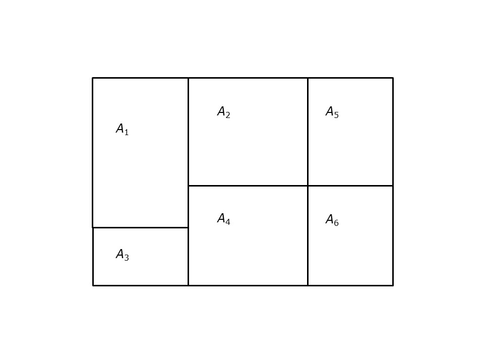
FIGURE 21.1: Simple zoning system
We can devise a way of establishing proximity between areas as follows: if points are selected in such a way that they are on the overlapping edges of two contiguous areas, the distance between these two areas clearly is zero, and they must be proximate.
This criterion to define proximity is called adjacency. Adjacency means that two zones share a common edge. This is conventionally called the rook criterion, after chess, in which the piece called the rook can move only orthogonally (in the vertical and horizontal directions). The rook criterion, however, would dictate that zones \(A_2\) and \(A_6\) are not proximate, despite being closer than \(A_2\) and \(A_3\).
When this criterion is expanded to allow contact at a single point between zones (say, the corner between \(A_2\) and \(A_6\)), the adjacency criterion is called queen, again, for the chess piece that moves both orthogonally and diagonally.
If we accept adjacency as a reasonable way of expressing relationships of proximity between areas, what we need is a way of coding relationships of adjacency in a way that is convenient and amenable to manipulation for data analysis.
One of the most widely used tools to code proximity in area data is the spatial weights matrix.
21.5 Spatial Weights Matrices
A spatial weights matrix is an arrangement of values (or weights) for all pairs of zones in a system. For instance, in a zoning system such as shown in Figure 1, with 6 zones, there will be \(6 \times 6\) such weights. The weights are organized by rows, in such a way that each zone has a corresponding row of weights. For example, zone \(A_1\) in Figure 1 has the following weights, one for each zone in the system: \[ w_{1\cdot} = [w_{11}, w_{12}, w_{13}, w_{14}, w_{15}, w_{16}] \]
The values of the weights depend on the adjacency criterion adopted. The simplest coding scheme is when we assign a value of 1 to pairs of zones that are adjacent, and a value of 0 to pairs of zones that are not.
Lets formalize the two criteria mentioned above:
- Rook criterion
\[ w_{ij}=\bigg\{\begin{array}{l l} 1\text{ if } A_i \text{ and } A_j \text{ share an edge}\\ 0\text{ otherwise}\\ \end{array} \] If rook adjacency is used, the weights for zone \(A_6\) are as follows: \[ w_{6\cdot} = [0, 0, 0, 1, 1, 0]. \]
As you can see, the adjacent areas from the perspective of \(A_6\) are \(A_4\) and \(A_5\) by virtue of sharing an edge. These two areas receive weights of 1. On the other hand, \(A_1\), \(a_2\), and \(A_3\) are not adjacent, and therefore receive a weight of zero. Notice how the weight \(w_{66}\) is set to zero. By convention, an area is not its own neighbor!
- Queen criterion
\[ w_{ij}=\bigg\{\begin{array}{l l} 1\text{ if } A_i \text{ and } A_j \text{ share an edge or a vertex}\\ 0\text{ otherwise}\\ \end{array} \]
If queen adjacency is used, the weights for zone \(A_6\) are as follows: \[ w_{6\cdot} = [0, 1, 0, 1, 1, 0]. \]
As you can see, the adjacent areas from the perspective of \(A_6\) are \(A_4\) and \(A_5\) (by virtue of sharing an edge), and \(A_2\) (by virtue of sharing a vertex). These three areas receive weights of 1. On the other hand, \(A_1\) and \(A_3\) are not adjacent, and therefore receive a weight of zero. Again, weight \(w_{66}\) is set to zero.
The set of weights above define the neighborhood of \(A_6\).
The spatial weights matrix for the whole system in Figure 1 is as follows: \[ \textbf{W}=\left (\begin{array}{c c c c c c} 0 & 1 & 1 & 1 & 0 & 0\\ 1 & 0 & 0 & 1 & 1 & 1\\ 1 & 0 & 0 & 1 & 0 & 0\\ 1 & 1 & 1 & 0 & 1 & 1\\ 0 & 1 & 0 & 1 & 0 & 1\\ 0 & 1 & 0 & 1 & 1 & 0\\ \end{array} \right). \]
Compare the matrix to the zoning system. The spatial weights matrix has the following properties:
The main diagonal elements of the matrix are all zeros (no area is its own neighbor).
Each zone has a row of weights in the matrix: row number one corresponds to \(A_1\), row number two corresponds to \(A_2\), and so on.
Likewise, each zone has a column of weights.
The sum of all values in a row gives the total number of neighbors for a zone. That is: \[ \text{The total number of neighbors of } A_i \text{ is given by: }\sum_{j=1}^{n}{w_{ij}} \]
The spatial weights matrix is often processed to obtain a row-standardized spatial weights matrix. This procedure consists of dividing every weight by the sum of its corresponding row (i.e., by the total number of neighbors of the zone), as follows: \[ w_{ij}^{st}=\frac{w_{ij}}{\sum_{j=1}^n{w_{ij}}} \]
The row-standardized weights matrix for the system in Figure 1 is: \[ \textbf{W}^{st}=\left (\begin{array}{c c c c c c} 0 & 1/3 & 1/3 & 1/3 & 0 & 0\\ 1/4 & 0 & 0 & 1/4 & 1/4 & 1/4\\ 1/2 & 0 & 0 & 1/2 & 0 & 0\\ 1/5 & 1/5 & 1/5 & 0 & 1/5 & 1/5\\ 0 & 1/3 & 0 & 1/3 & 0 & 1/3\\ 0 & 1/3 & 0 & 1/3 & 1/3 & 0\\ \end{array} \right). \]
The row-standardized spatial weights matrix has the following properties:
Each weight now represents the proportion of a neighbor out of the total of neighbors. For instance, since the total of neighbors of \(A_1\) is 3, each neighbor contributes 1/3 to that total.
The sum of all weights over a row equals 1, or 100% of all neighbors for that zone.
21.6 Creating Spatial Weights Matrices in R
Coding spatial weights matrices by hand is a tedious and error-prone process. Fortunately, functions to generate them exist in R. The package spdep in particular has a number of useful utilities for working with spatial weights matrices.
The first step to create a spatial weights matrix is to find the neighbors (i.e., areas adjacent to) for each area. The function poly2nb is used for this (note that the default adjacency criterion is queen):
# The function `poly2nb()` takes an object of class "Spatial" with polygons, and finds the neighbors

Hamilton_CT.nb <- poly2nb(pl = Hamilton_CT, queen = TRUE)
The value (output) of the function is an object of class nb:
## [1] "nb"The function summary() applied to an object of this class gives some useful information about the neighbors in the region, including the number of zones in this system (\(188\)), the total number of neighbors (\(1,180\)), and the percentage of neighbors out of all pairs of areas (3.34%; conversely, 96.66% of all possible zone pairs are not neighbors!) Other information includes the distribution of neighbors (3 zones have two neighbors, 8 zones have three neighbors, 22 zones have four neighbors, and so on):
## Neighbour list object:
## Number of regions: 188
## Number of nonzero links: 1180
## Percentage nonzero weights: 3.338615
## Average number of links: 6.276596
## Link number distribution:
##
##  2  3  4  5  6  7  8  9 10 11 12 14
##  3  8 22 32 35 45 30  6  1  1  4  1
## 3 least connected regions:
## 174 175 188 with 2 links
## 1 most connected region:
## 33 with 14 links
The nb object is a list that contains the neighbors for each zone. For instance, the neighbors of census tract 5370001.01 (the first tract in the dataframe) are the following tracts:
# Here, the indexing works by making reference to the first set of zone in `Hamilton_CT.nb` and then using those values to retrieve the census tract identifiers from our `Hamilton_CT` dataframe

Hamilton_CT$TRACT[Hamilton_CT.nb[[1]]]
## [1] "5370120.02" "5370122.01" "5370122.02" "5370124.00" "5370142.01"
## [6] "5370133.01" "5370130.03"The list of neighbors can be converted into a list of entries in a spatial weights matrix \(W\) by means of the function nb2listw (for “neighbors to matrix W in list form”):
We can use base R functions to visualize the neighbors (adjacent) areas in our system:
# Plot the geometry of the zoning system
plot(Hamilton_CT |>
       st_geometry(), border = "gray")
# Plot the neighbhorhood relationships; this uses two arguments: the `nb` class object and the coordinates of the centroids of the zoning system
plot(Hamilton_CT.nb,
     Hamilton_CT |>
       st_centroid() |>
       st_coordinates(),
     # Add to the previous plot
     add = TRUE,
     col = "red")
## Warning: st_centroid assumes attributes are constant over geometries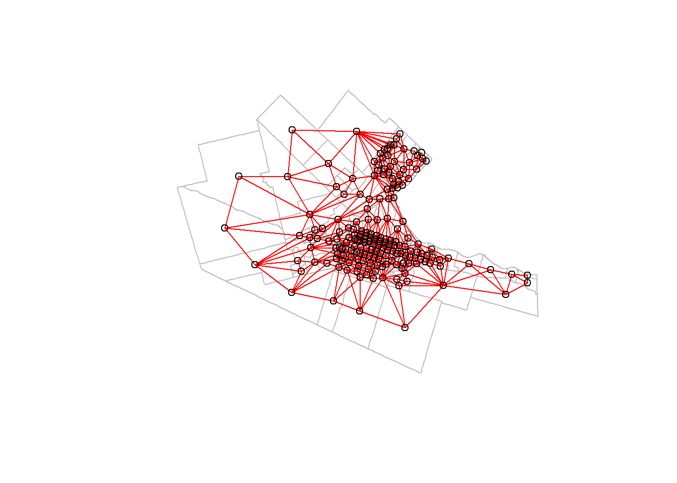
21.7 Spatial Moving Averages
The spatial weights matrix \(W\), and in particular its row-standardized version \(W^{st}\), is useful to calculate a spatial statistic, the spatial moving average.
The spatial moving average is a variation of the mean statistic: in fact, it is a weighted average, calculated using the spatial weights. Recall that the mean is calculated as the sum of all relevant values divided by the number of values summed. In the case of spatial data, the mean is what we would call a global statistic, since it is calculated using all data for a region: \[ \bar{x}=\frac{1}{n}\sum_{j=1}^{n}{x_j} \] where \(\bar{x}\) (read x-bar) is the mean of all values of x.
A spatial moving average is calculated in the same way, but for each area, and based only on the values of proximate areas: \[ \bar{x_i}=\frac{1}{n_i}\sum_{j\in N(i)}{x_j} \] where \(n_i\) is the number of neighbors of \(A_i\), and the sum is only for \(x_j\) that are in the neighborhood of i (\(j\in N(i)\) is read “j in the neighborhood of i”).
We can illustrate the way spatial moving averages work by making reference again to Figure 1.
Consider zone \(A_1\). The spatial weights matrix indicates that the neighborhood of \(A_1\) consists of three areas: \(A_2\), \(A_3\), and \(A_4\). Therefore \(n_1=3\), and \(j\in N(1)\) are 2, 3, and 4.
The spatial moving average of \(A_1\) for a variable \(x\) would then be calculated as: \[ \bar{x}_1=\frac{x_2 + x_3 + x_4}{3} \]
Notice that another way of writing the spatial moving average expression is as follows, since membership in the neighborhood of \(i\) is implicit in the definition of \(w_{ij}\)! Since \(w_{ij}\) takes values of zero and one, the effect is to turn on and off the values of \(x\) depending on whether they are for areas adjacent to \(i\): \[ \bar{x}_i=\frac{1}{n_i}\sum_{j=1}^n{w_{ij}x_j} \]
This means that the spatial moving average of \(A_1\) for a variable \(x\) on this system can also be calculated using the spatial weights matrix as: \[ \bar{x}_1=\frac{w_{11}x_1 + w_{12}x_2 + w_{13}x_3 + w_{14}x_4 + w_{15}x_5 + w_{12}x_6}{3} \]
Substituting the spatial weights: \[ \bar{x}_1=\frac{0x_1 + 1x_2 + 1x_3 + 1x_4 + 0x_5 + 0x_6}{3} = \frac{x_2 + x_3 + x_4}{3} \]
In other words, the spatial weights can be used directly in the calculation of spatial moving averages.
Further, notice that: \[ n_i=\sum_{j=1}^{n}w_{ij} \] which is simply the total number of neighbors of \(A_i\), and the value we used to row-standardize the spatial weights.
Since the row-standardized weights have already been divided by the number of neighbors, we can use them to express the spatial moving average as follows: \[ \bar{x}_i=\sum_{j=1}^{n}{w_{ij}^{st}x_j} \]
Continuing with this example, if we use the row-standardized weights, the spatial moving average at \(A_1\) is: \[ \bar{x}_i=0x_1 + \frac{1}{3}x_2 + \frac{1}{3}x_3 + \frac{1}{3}x_4 + 0x_5 + 0x_6 \] which is the same as: \[ \bar{x}_i=\frac{x_2 + x_3 + x_4}{3} \]
Consider the following map of Hamilton’s population density:
# You have seen previously how to create a choropleth map using quintiles. The first part of this is a choropleth map of population density

map <- ggplot(data = Hamilton_CT) +
  geom_sf(aes(fill = cut_number(Hamilton_CT$POP_DENSITY, 5),
                   POP_DENSITY = round(POP_DENSITY),
                   TRACT = TRACT),
               color = "black") +
  # For the example, two census tracts will be identified more explicitly
  # Next, we the function `filter()` to select census tract 5370142.02. We will color red the boundaries of this census tract
  geom_sf(data = filter(Hamilton_CT, TRACT == "5370142.02"),
               aes(POP_DENSITY = round(POP_DENSITY),
                   TRACT = TRACT),
               color = "red",
               weight = 3, fill = NA) +
    # We the function `filter()` again, now to select census tract 5370144.01. We will color green the boundaries of this census tract
  geom_sf(data = subset(Hamilton_CT, TRACT == "5370144.01"),
               aes(POP_DENSITY = round(POP_DENSITY),
                   TRACT = TRACT),
               color = "green",
               weight = 3, fill = NA) +
  # This selects a palette for the fill colors and changes the label for the legend
  scale_fill_brewer(palette = "YlOrRd") +
  labs(fill = "Pop Density") +
  coord_sf()

# The function `ggplotly()` takes a `ggplot2` object and creates an interactive map
ggplotly(map, tooltip = c("TRACT", "POP_DENSIT"))
Manually calculate the spatial moving average for tract 5370142.02 (with the red boundary) and tract (with the green boundary). Tip: hover over the tracts to see their population densities.
## [1] 63## [1] 76Spatial moving averages can be calculated in a straightforward way by means of the function lag.listw() function of the spdep package. This function uses a spatial weights matrix and automatically selects the row-standardized weights.
Here, we calculate the spatial moving average of population density:
And now we can plot the spatial moving average of population density. First we join this variable to our sf dataframe with the census tracts. The key for joining the two dataframes is the unique tract identifier :
Hamilton_CT <- left_join(Hamilton_CT,
                         data.frame(TRACT = Hamilton_CT$TRACT, POP_DENSITY.sma),
                         by = "TRACT")
And plot:
# In this chunk of code we create a choropleth map, but now of the spatial moving average of population density

# First map the spatial moving average of population density using quintiles
map.sma <- ggplot() +
  geom_sf(data = Hamilton_CT,
          aes(fill = cut_number(Hamilton_CT$POP_DENSITY.sma, 5),
              POP_DENSITY.sma = round(POP_DENSITY.sma),
              TRACT = TRACT),
          color = "black") +
  # Select and plot census tract 5370142.02 and color its boundaries in red
  geom_sf(data = filter(Hamilton_CT, TRACT == "5370142.02"),
          aes(POP_DENSITY.sma = round(POP_DENSITY.sma),
              TRACT = TRACT),
          color = "red",
          weight = 3, fill = NA) +
  # Select and plot census tract 5370144.01 and color its boundaries in green
  geom_sf(data = filter(Hamilton_CT, TRACT == "5370144.01"),
          aes(POP_DENSITY.sma = round(POP_DENSITY.sma),
              TRACT = TRACT),
          color = "green",
          weight = 3, fill = NA) +
  # Embellish the map with a color palette to your taste and labels
  scale_fill_brewer(palette = "YlOrRd") +
  labs(fill = "Pop Density SMA") +
  coord_sf()

# Again, `ggplotly()` takes the `ggplot2` object and creates an interactive map
ggplotly(map.sma, tooltip = c("TRACT", "POP_DENSIT.sma"))
Verify that your manual calculations for the two tracts above are correct. What differences do you notice between the map of population density and the map of spatial moving averages of population density?
21.8 Other Criteria for Coding Proximity
Adjacency is not the only criterion that can be used for coding proximity.
Occasionally, the distance between areas is calculated by using the centroids of the areas as their representative points. A centroid is simply the mean of the coordinates of the edges of an area, and in this way represent the “center of gravity” of the area.
The inter-centroid distance allows us to define additional criteria for proximity, including neighbors within a certain distance threshold, and \(k\)-nearest neighbors.
- Distance-based criterion
\[ w_{ij}=\bigg\{\begin{array}{l l} 1\text{ if inter-centroid distance } d_{ij}\leq \delta\\ 0\text{ otherwise}\\ \end{array} \] where \(\delta\) is a distance threshold.
Distance-based nearest neighbors can be obtained in R by means of the function dnearneigh().
To implement this criterion we need to find the centroids of the polygons with st_centroid() and then extract the coordinates of the centroids with st_coordinates():
## Warning: st_centroid assumes attributes are constant over geometriesWe can create a nearest neighbors object nb using two threshold distances, a minimum and a maximum distance value. In this example we will consider that the neighbors of zone \(A_i\) are all zones \(A_j\) whose centroids are within \(0\) and \(5,000\) meters of the centroid of \(A_i\):
## Warning in dnearneigh(CT_centroids, d1 = 0, d2 = 5000): neighbour object has 9
## sub-graphs
We can visualize the neighbors (adjacent) areas:
plot(Hamilton_CT |>
       st_geometry(),
     border = "gray")
plot(Hamilton_CT.dnb,
     CT_centroids,
     col = "red",
     add = TRUE)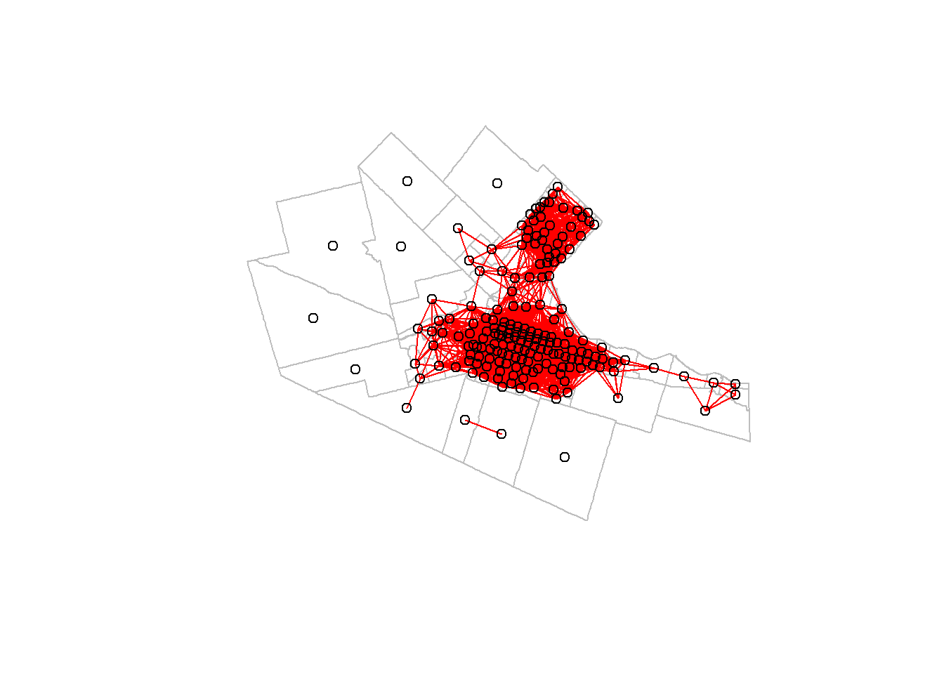
Try changing the distance threshold to see how different neighborhoods are defined.
- \(k\)-nearest neighbors
A potential disadvantage of using a distance-based criterion is that for zoning systems with areas of vastly different sizes, small areas will end up having many neighbors, whereas large areas will have few or none.
The criterion of \(k\)-nearest neighbors allows for some adaptation to the size of the areas. Under this criterion, all zones have the exact same number of neighbors, but the geographical extent of the neighborhood may (and likely will) change. The criterion is defined as follows: \[ w_{ij}=\bigg\{\begin{array}{l l} 1\text{ if } A_j \text{ is one of } k\text{-nearest neighbors of } A_i\\ 0\text{ otherwise}\\ \end{array} \]
In R, \(k\)-nearest neighbors can be obtained by means of the function knearneigh(), and the arguments include the value of \(k\):
We can again visualize the neighbors (“adjacent”) areas:
plot(Hamilton_CT |>
       st_geometry(),
     border = "gray")
plot(Hamilton_CT.knb,
     CT_centroids,
     col = "red",
     add = TRUE)
Try changing the value of k to see how the neighborhoods change.
This chapter has equipped you to define various forms of proximity for area data. You have also seen how spatial moving averages can be calculated using row-standardized spatial weights matrices.