Chapter 4 Activity: Statistical Maps I
NOTE: The source files for this book are available with companion package {isdas}. The source files are in Rmarkdown format and packed as templates. These files allow you execute code within the notebook, so that you can work interactively with the notes.
4.1 Housekeeping Questions
Answer the following questions:
What are the office hours of your instructor this term?
How are assignments graded?
What is the policy for late assignments in this course?
4.2 Learning Objectives
In this activity you will:
- Discuss statistical maps and what makes them interesting.
4.3 Preliminaries
In the practice that preceded this activity, you used ggmap to create a proportional symbol map, a mapping technique used in spatial statistics for visualization of geocoded event information. As well, you implemented a simple technique called kernel analysis to the map to explore the distribution of events in the case of the cholera outbreak of Soho in London in 1854. Geocoded events are often called point patterns, so with the cholera data you were working with a point pattern.
In this activity, we will map another type of spatial data, called areal data. Areas are often administrative or political jurisdictions.
it is good practice to begin with a clean session to make sure that you do not have extraneous items there when you begin your work. The best practice is to restart the R session, which can be accomplished for example with command/ctrl + shift + F10. An alternative to only purge user-created objects from memory is to use the R command rm (for “remove”), followed by a list of items to be removed:
Note that ls() lists all objects currently on the workspace.
Load the libraries you will use in this activity:
## Warning: replacing previous import 'dplyr::lag' by 'stats::lag' when loading
## 'isdas'
## Warning: replacing previous import 'plotly::filter' by 'stats::filter' when
## loading 'isdas'## Linking to GEOS 3.12.1, GDAL 3.8.4, PROJ 9.4.0; sf_use_s2() is TRUE## ── Attaching core tidyverse packages ──────────────────────── tidyverse 2.0.0 ──
## ✔ dplyr 1.1.4 ✔ readr 2.1.5
## ✔ forcats 1.0.0 ✔ stringr 1.5.1
## ✔ ggplot2 3.5.1 ✔ tibble 3.2.1
## ✔ lubridate 1.9.4 ✔ tidyr 1.3.1
## ✔ purrr 1.0.2## ── Conflicts ────────────────────────────────────────── tidyverse_conflicts() ──
## ✖ dplyr::filter() masks stats::filter()
## ✖ dplyr::lag() masks stats::lag()
## ℹ Use the conflicted package (<http://conflicted.r-lib.org/>) to force all conflicts to become errors4.4 Creating a simple thematic map
If you successfully loaded package isdas a dataset called HamiltonDAs should be available for analysis:
Check the class of this object:
## [1] "sf" "data.frame"As you can see, this is an object of class sf, which stands for simple features. Objects of this class are used in the R package sf (see here) to implement standards for spatial objects.
You can examine the contents of the dataset by means of head (which will show the top rows):
## Simple feature collection with 6 features and 7 fields
## Geometry type: MULTIPOLYGON
## Dimension:     XY
## Bounding box:  xmin: 563306.2 ymin: 4777681 xmax: 610844.5 ymax: 4793682
## Projected CRS: NAD83 / UTM zone 17N
##     ID GTA06       VAR1      VAR2      VAR3      VAR4      VAR5
## 1 2671  5030 0.74650172 0.2596975 0.6361925 0.2290084 0.7223464
## 2 2716  5077 0.78107142 0.4413119 0.5690740 0.8997258 0.4163702
## 3 2710  5071 0.78824936 0.4632757 0.4197216 0.1619401 0.3052948
## 4 2745  5108 0.82064933 0.6365193 0.9504535 0.4992477 0.6046399
## 5 2810  5177 0.09131849 0.4455965 0.3539603 0.4919869 0.6366968
## 6 2740  5103 0.22257665 0.6288826 0.1341962 0.6635202 0.4429712
##                         geometry
## 1 MULTIPOLYGON (((605123.4 47...
## 2 MULTIPOLYGON (((606814 4784...
## 3 MULTIPOLYGON (((605293 4785...
## 4 MULTIPOLYGON (((607542.7 47...
## 5 MULTIPOLYGON (((564681.8 47...
## 6 MULTIPOLYGON (((574373.4 47...
Or obtain the summary statistics by means of summary:
##        ID          GTA06          VAR1             VAR2             VAR3
##  2299   :  1   4050   :  1   Min.   :0.0000   Min.   :0.0000   Min.   :0.0000
##  2300   :  1   4051   :  1   1st Qu.:0.3680   1st Qu.:0.3800   1st Qu.:0.3521
##  2301   :  1   4052   :  1   Median :0.5345   Median :0.4937   Median :0.5699
##  2302   :  1   4053   :  1   Mean   :0.5241   Mean   :0.4966   Mean   :0.5548
##  2303   :  1   4054   :  1   3rd Qu.:0.6938   3rd Qu.:0.6091   3rd Qu.:0.7378
##  2304   :  1   4055   :  1   Max.   :1.0000   Max.   :1.0000   Max.   :1.0000
##  (Other):291   (Other):291
##       VAR4             VAR5                 geometry
##  Min.   :0.0000   Min.   :0.0000   MULTIPOLYGON :297
##  1st Qu.:0.2989   1st Qu.:0.2998   epsg:26917   :  0
##  Median :0.5476   Median :0.4810   +proj=utm ...:  0
##  Mean   :0.5325   Mean   :0.5001
##  3rd Qu.:0.7894   3rd Qu.:0.6915
##  Max.   :1.0000   Max.   :1.0000
##
The above will include a column for the geometry of the spatial features.
The dataframe includes all Dissemination Areas (or DAs for short) for the Hamilton Census Metropolitan Area in Canada. DAs are a type of geography used by the Census of Canada, in fact the smallest geography that is publicly available.
To create a simple map we can use ggplot2, which previously we used to map points. Now, the geom for objects of class sf can be used to plot areas. To create such a map, we layer a geom object of type sf on a ggplot2 object. For instance, to plot the DAs:
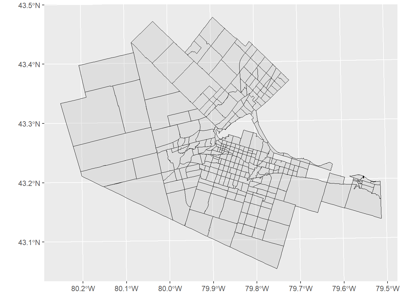
We selected color “black” for the polygons, with a transparency alpha = 0.3 (alpha = 0 is completely transparent, alpha = 1 is completely opaque, try it!), and line size 0.3.
This map only shows the DAs, which is nice. However, as you saw in the summary of the dataframe above, in addition to the geometric information, a set of (generic) variables is also included, called VAR1, VAR2,…, VAR5.
Thematic maps can be created using these variables. The next chunk of code plots the DAs and adds info. The fill argument is used to select a variable to color the polygons. The function cut_number is used to classify the values of the variable in \(k\) groups of equal size, in this case 5 (notice that the lines of the polygons are still black). The scale_fill_brewer function can be used to select different palettes or coloring schemes):
ggplot(HamiltonDAs) +
  geom_sf(aes(fill = cut_number(HamiltonDAs$VAR1, 5)), color = "black", alpha = 1, size = .3) +
  scale_fill_brewer(palette = "Reds") +
  coord_sf() +
  labs(fill = "Variable")
## Warning: Use of `HamiltonDAs$VAR1` is discouraged.
## ℹ Use `VAR1` instead.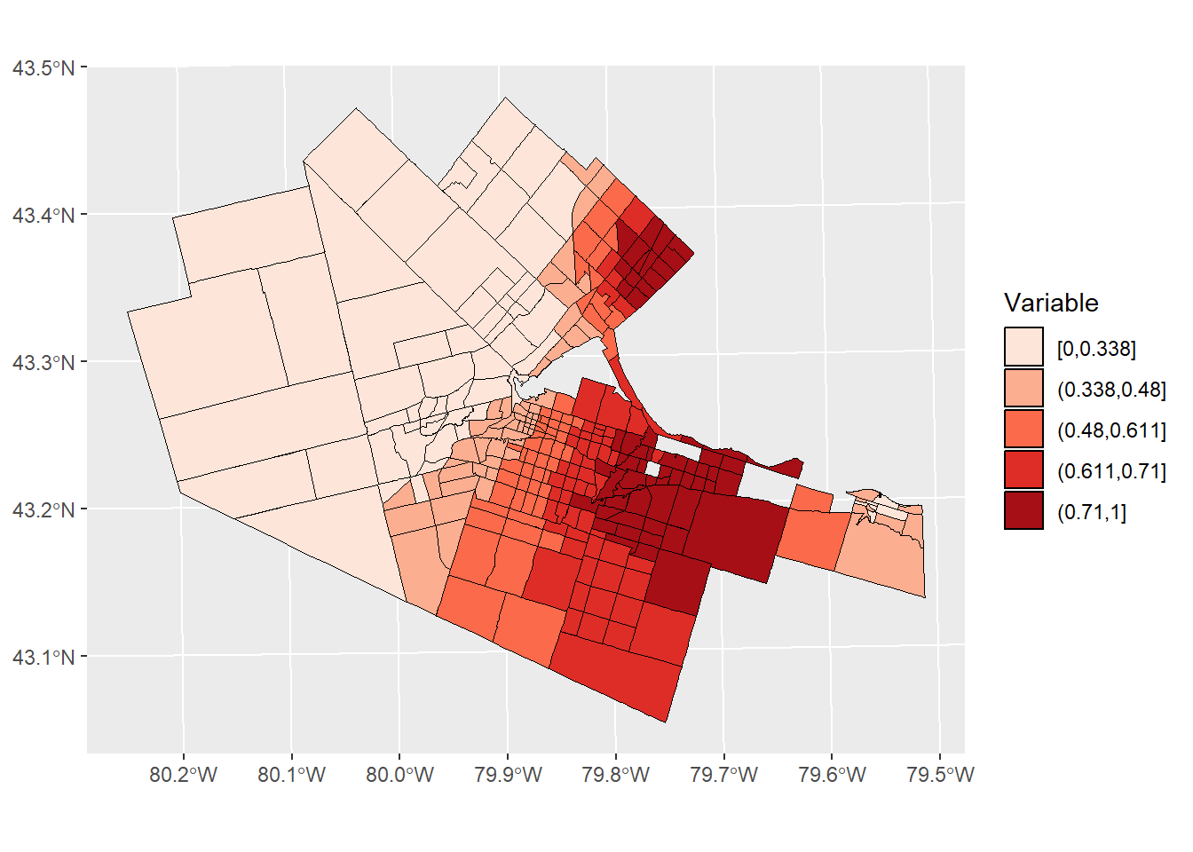
Now you have seen how to create a thematic map with polygons (areal data), you are ready for the following activity.
4.5 Activity
NOTE: Activities include technical “how to” tasks/questions. Usually, these ask you to practice using the software to organize data, create plots, and so on in support of analysis and interpretation. The second type of questions ask you to activate your brainware and to think geographically and statistically.
Activity Part I
- Create thematic maps for variables VAR1 through VAR5 in the dataframe
HamiltonDAs. Remember that you can introduce new chunks of code.
Activity Part II
- Imagine that the maps you produced in the first question were found, and for some reason the variables were not labeled. They may represent income, or population density, or something else. Which of the five maps you just created is more interesting? Rank the five maps from most to least interesting. Explain the reasons for your ranking.