Figurative mosaics with flexible tiles
Source:vignettes/articles/a03-figurative-mosaics.Rmd
a03-figurative-mosaics.RmdFlexible Truchet tiles are a fantastic tool for creating figurative mosaics. The technique was described by Bosch and Colley in a 2013 paper in the Journal of Mathematics and the Arts.
This article shows how to use {truchet} to generate figurative mosaics. In addition to {truchet}, we need {dplyr}, {ggplot2}, and {imager}, {purrr}, and {sf}:
library(dplyr)
#>
#> Attaching package: 'dplyr'
#> The following objects are masked from 'package:stats':
#>
#>     filter, lag
#> The following objects are masked from 'package:base':
#>
#>     intersect, setdiff, setequal, union
library(ggplot2)
library(imager)
#> Loading required package: magrittr
#>
#> Attaching package: 'imager'
#> The following object is masked from 'package:magrittr':
#>
#>     add
#> The following object is masked from 'package:dplyr':
#>
#>     where
#> The following objects are masked from 'package:stats':
#>
#>     convolve, spectrum
#> The following object is masked from 'package:graphics':
#>
#>     frame
#> The following object is masked from 'package:base':
#>
#>     save.image
library(purrr)
#>
#> Attaching package: 'purrr'
#> The following object is masked from 'package:magrittr':
#>
#>     set_names
library(sf)
#> Linking to GEOS 3.12.1, GDAL 3.8.4, PROJ 9.4.0; sf_use_s2() is TRUE
library(truchet)
The basic idea is as follows.
A mosaic can be made of a collection of tiles, possibly in regular arrangements. Take the four elemental Truchet tiles, so-called tiles A, B, C, and D:
# Tiles types
tile_types <- data.frame(type = c("Al", "Bl", "Cl", "Dl")) %>%
  mutate(x = c(1, 2.5, 1, 2.5),
         y = c(2.5, 2.5, 1, 1),
         b = 1/2)

# Elements for assembling the mosaic
x_c <- tile_types$x
y_c <- tile_types$y
type <- as.character(tile_types$type)
b <- tile_types$b

pmap_dfr(list(x_c, y_c, type, b), st_truchet_flex) %>%
  ggplot() +
  geom_sf(aes(fill = color),
          color = "black",
          size = 2) +
  geom_text(data = tile_types,
            aes(x = x,
                y = y,
                label = c("A", "B", "C", "D")),
            nudge_y = 0.6) +
  scale_fill_distiller(direction = 1) +
  theme_void() +
  theme(legend.position = "none")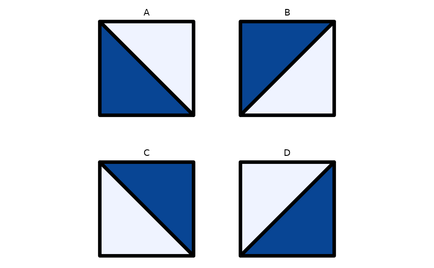
A simple arrangement of a 1 by 1 matrix is just one tile repeated in the mosaic, for example “A”. This is what Truchet denominated “Design A”:
# Tiles types
tile_types <- data.frame(type = c("Al", "Al", "Al", "Al")) %>%
  mutate(x = c(1, 2, 1, 2),
         y = c(2, 2, 1, 1),
         b = 1/2)

# Elements for assembling the mosaic
x_c <- tile_types$x
y_c <- tile_types$y
type <- as.character(tile_types$type)
b <- tile_types$b

pmap_dfr(list(x_c, y_c, type, b), st_truchet_flex) %>%
  ggplot() +
  geom_sf(aes(fill = color),
          color = "black",
          size = 2) +
  geom_text(data = tile_types,
            aes(x = x,
                y = y,
                label = c("Design A", "", "", "")),
            nudge_y = 0.6) +
  scale_fill_distiller(direction = 1) +
  theme_void() +
  theme(legend.position = "none")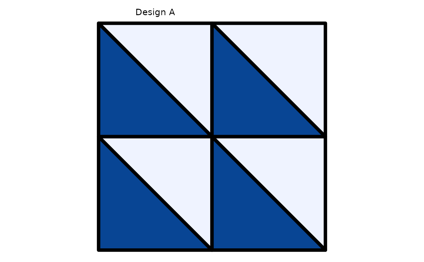
The basic matrix can also be , for example: This is Truchet’s Design C:
# Tiles types
tile_types <- data.frame(type = c("Al", "Cl", "Cl", "Al")) %>%
  mutate(x = c(1, 2, 1, 2),
         y = c(2, 2, 1, 1),
         b = 1/2)

# Elements for assembling the mosaic
x_c <- tile_types$x
y_c <- tile_types$y
type <- as.character(tile_types$type)
b <- tile_types$b

pmap_dfr(list(x_c, y_c, type, b), st_truchet_flex) %>%
  ggplot() +
  geom_sf(aes(fill = color),
          color = "black",
          size = 2) +
  geom_text(data = tile_types,
            aes(x = x,
                y = y,
                label = c("Design C", "", "", "")),
            nudge_y = 0.6) +
  scale_fill_distiller(direction = 1) +
  theme_void() +
  theme(legend.position = "none")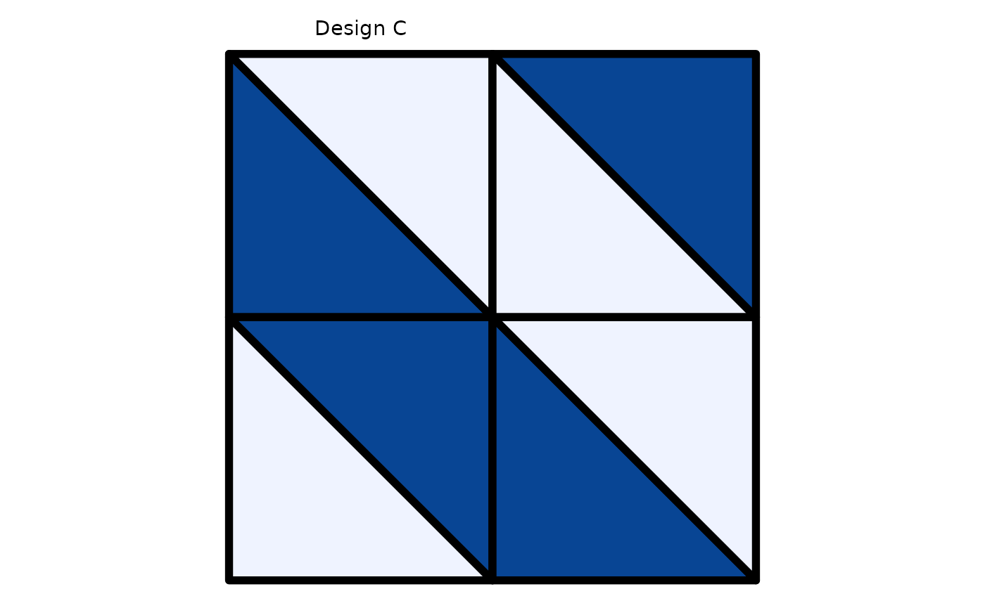
Judicious use of the parameter to control the fold of the boundary of each tile changes the “darkness” of the tile. For example, this is Design C with a lighter color (b = 1/3):
# Tiles types
tile_types <- data.frame(type = c("Al", "Cl", "Cl", "Al")) %>%
  mutate(x = c(1, 2, 1, 2),
         y = c(2, 2, 1, 1),
         b = c(1/3, 1 - 1/3, 1 - 1/3, 1/3))

# Elements for assembling the mosaic
x_c <- tile_types$x
y_c <- tile_types$y
type <- as.character(tile_types$type)
b <- tile_types$b

pmap_dfr(list(x_c, y_c, type, b), st_truchet_flex) %>%
  ggplot() +
  geom_sf(aes(fill = color),
          color = "black",
          size = 2) +
  geom_text(data = tile_types,
            aes(x = x,
                y = y,
                label = c("Design C with b = 1/3", "", "", "")),
            nudge_y = 0.6) +
  scale_fill_distiller(direction = 1) +
  theme_void() +
  theme(legend.position = "none")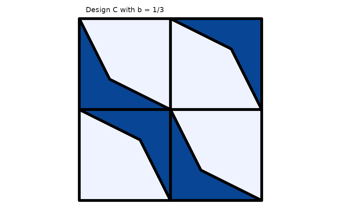
This is Design C with a darker color (b = 2/3):
# Tiles types
tile_types <- data.frame(type = c("Al", "Cl", "Cl", "Al")) %>%
  mutate(x = c(1, 2, 1, 2),
         y = c(2, 2, 1, 1),
         b = c(2/3, 1 - 2/3, 1 - 2/3, 2/3))

# Elements for assembling the mosaic
x_c <- tile_types$x
y_c <- tile_types$y
type <- as.character(tile_types$type)
b <- tile_types$b

pmap_dfr(list(x_c, y_c, type, b), st_truchet_flex) %>%
  ggplot() +
  geom_sf(aes(fill = color),
          color = "black",
          size = 2) +
  geom_text(data = tile_types,
            aes(x = x,
                y = y,
                label = c("Design C with b = 1/3", "", "", "")),
            nudge_y = 0.6) +
  scale_fill_distiller(direction = 1) +
  theme_void() +
  theme(legend.position = "none")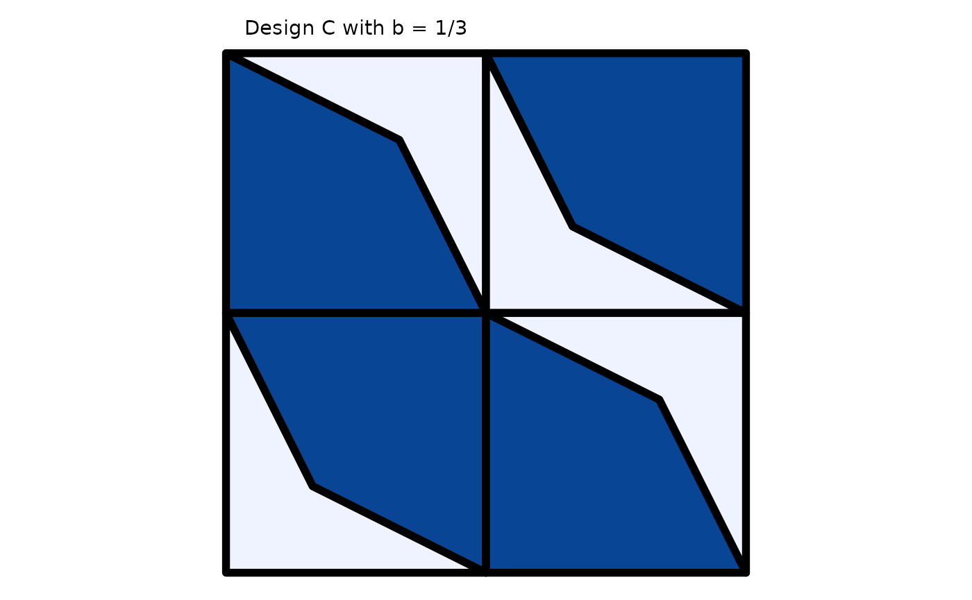
Notice that the parameter alternates between b and
1 - b to ensure that the four tiles in this
matrix look uniformly darker. Since b takes values between
0 and 1 (it represents a proportion of the length of the diagonal of the
tile), an underlying variable can be used to modify the “darkness” of
the tiles locally. In this way, an image in grayscale can give those
values, as illustrated next.
This example uses an image of Elvis in the jail. Read the image using
imager::load.image():
elvis <- imager::load.image(system.file("extdata",
                                "elvis.jpg",
                                package = "truchet"))
The size of the image is and has three colour channels.
elvis
#> Image. Width: 1031 pix Height: 1280 pix Depth: 1 Colour channels: 3
This is Elvis doing the jailhouse rock:
plot(elvis)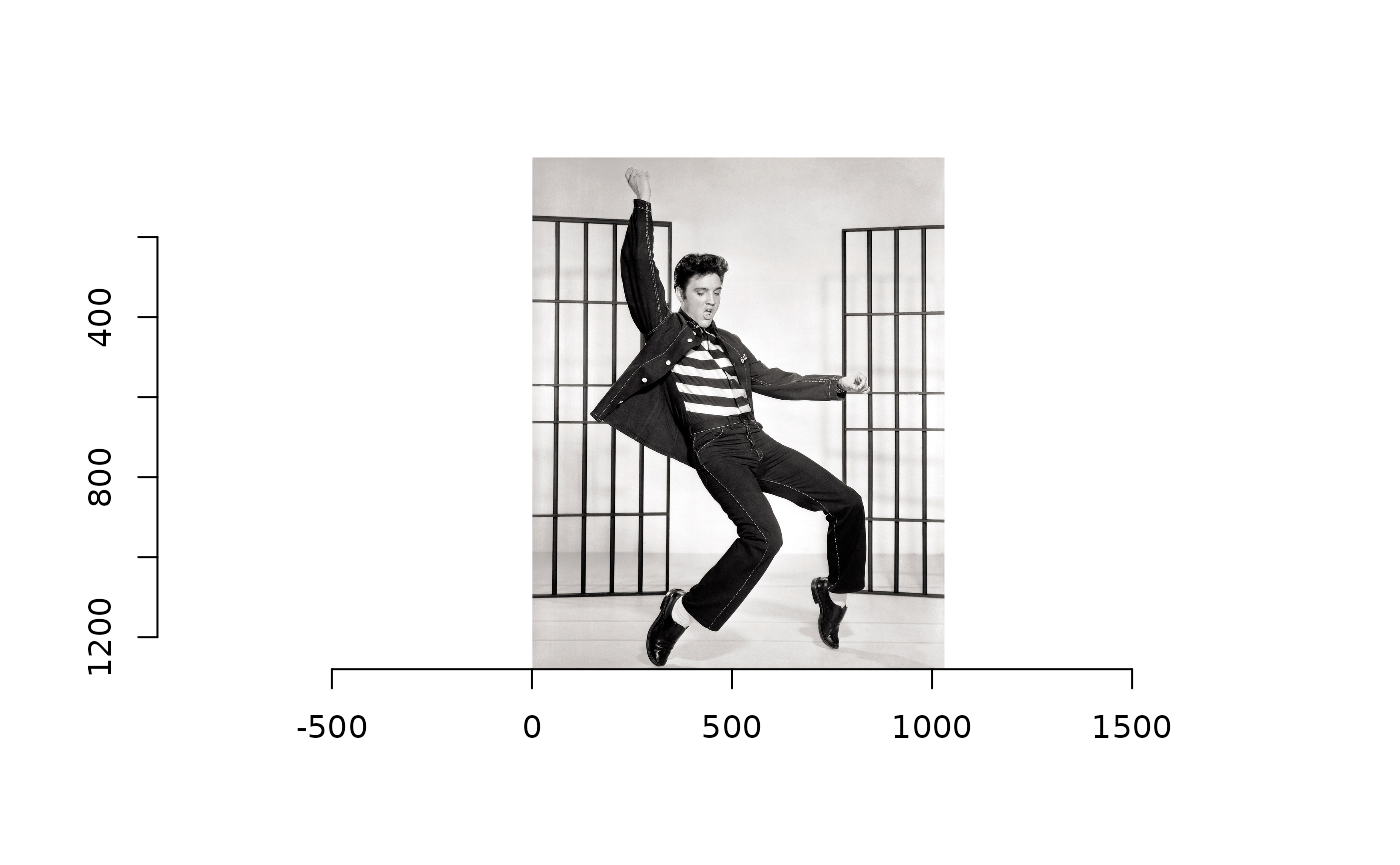
The size of the image means that there are 1.31968^{6} pixels. Creating an image with all these pixels is very lengthy, and not very interesting because the high resolution means that the figurative aspect of the mosaic is lost. Instead of working with the original image, here we scale it so that its width is 200 pixels:
elvis_rs <- imresize(elvis, scale = 1/15, interpolation = 6)Now the size of the image is and consists of only 4636 pixels. Clearly, the resolution is much lower and a lot of detail is lost, but that is part of the point of doing a figurative mosaic:
plot(elvis_rs)
To use this image we need to change its color map to grayscale and
also to transform from class cimg/imager_array
to data frame:
elvis_df <- elvis_rs %>%
  grayscale() %>%
  as.data.frame()
This data frame now includes the coordinates of the pixels (but note
that the y axis is reversed due to the convention to index pixels in an
image). In addition, the column value gives the shades of
gray, with 0 = white and 1 = black:
summary(elvis_df)
#>        x            y             value
#>  Min.   : 1   Min.   : 1.00   Min.   :0.002297
#>  1st Qu.:16   1st Qu.:19.75   1st Qu.:0.557348
#>  Median :31   Median :38.50   Median :0.807564
#>  Mean   :31   Mean   :38.50   Mean   :0.682023
#>  3rd Qu.:46   3rd Qu.:57.25   3rd Qu.:0.888449
#>  Max.   :61   Max.   :76.00   Max.   :1.000000
Now we can use this data frame to design the mosaic. Here we use
Design C. The modulus operation is used to create a checkerboard pattern
of tiles A and C that replicates the matrix
,
and also to adjust parameter b when creating the tiles:
df <- elvis_df %>%
  # Reverse the y axis
  mutate(y = -(y - max(y)),
         # The modulus of x + y can be used to create a checkerboard pattern
         tiles = case_when((x + y) %% 2 == 0 ~ "Al",
                           (x + y) %% 2 == 1 ~ "Cl"),
         b = case_when((x + y) %% 2 == 0 ~ 1 - value,
                       (x + y) %% 2 == 1 ~ value))
Function st_truchet_fm() is used to create a mosaic of
flexible tiles. Column b is scaled to avoid completely
white or completely black tiles:
# Start a timer
start_time <- Sys.time()

# Assemble mosaic
mosaic <- st_truchet_fm(df = df %>%
                          mutate(b = b * 0.99 + 0.001))

# End timer
end_time <- Sys.time()

# Calculate time
end_time - start_time
#> Time difference of 43.64118 secs
It takes two or three minutes to process an image of 61 by 76 pixels.
Since the mosaic is a simple features data frame it can be plotted
using geom_sf() in {ggplot2}:
mosaic %>%
  ggplot() +
  geom_sf(aes(fill = color),
          color = NA) +
  scale_fill_distiller(direction = 1) +
  coord_sf(expand = FALSE) +
  theme_void() +
  theme(legend.position = "none")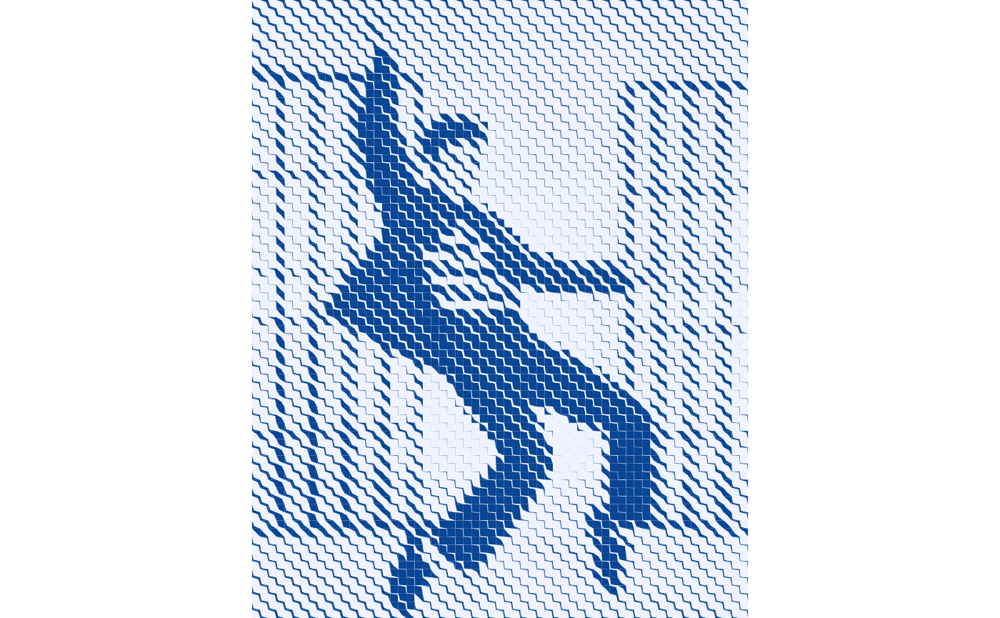
Other designs can be used. Truchet’s Design D results from the following matrix:
This is a windmill-like set of 4 tiles:
# Tiles types
tile_types <- data.frame(type = c("Bl", "Al", "Cl", "Dl")) %>%
  mutate(x = c(1, 2, 1, 2),
         y = c(2, 2, 1, 1),
         b = 1/2)

# Elements for assembling the mosaic
x_c <- tile_types$x
y_c <- tile_types$y
type <- as.character(tile_types$type)
b <- tile_types$b

pmap_dfr(list(x_c, y_c, type, b), st_truchet_flex) %>%
  ggplot() +
  geom_sf(aes(fill = color),
          color = "black",
          size = 2) +
  geom_text(data = tile_types,
            aes(x = x,
                y = y,
                label = c("Design D", "", "", "")),
            nudge_y = 0.6) +
  scale_fill_distiller(direction = 1) +
  theme_void() +
  theme(legend.position = "none")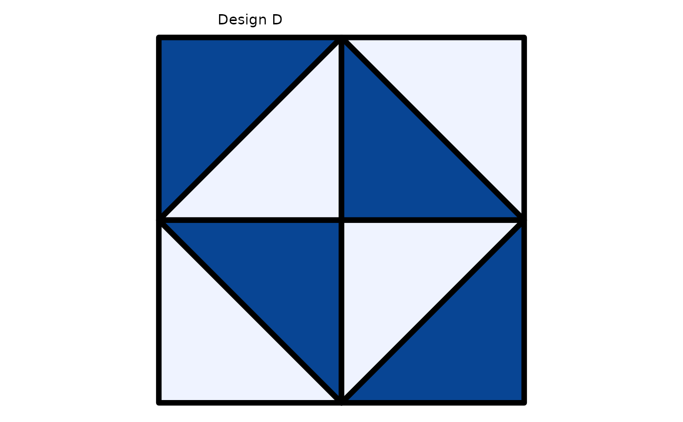
To illustrate this design, we will use the iconic image of Frida Kahlo:
frida <- load.image(system.file("extdata",
                                "frida.jpg",
                                package = "truchet"))
This is the source image:
plot(frida)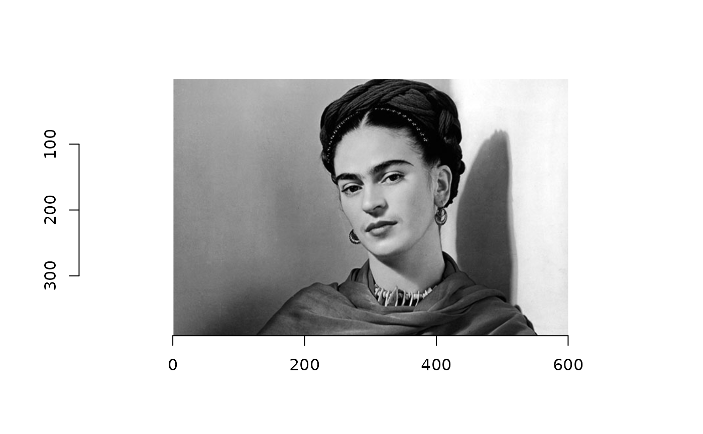
We can select part of the image, for instance to zoom in on the face:
The resolution may still be high for the mosaic, so we resize image:
frida_rs <- imresize(frida_sel, scale = 1/5, interpolation = 6)As before, we convert to grayscale and then to data frame:
frida_df <- frida_rs %>%
  grayscale() %>%
  as.data.frame()
Creating this design is a little bit trickier. Notice the use of
dplyr::case_when() and the modulus operation to place the
tiles:
df <- frida_df %>%
  # Reverse the y axis
  mutate(y = -(y - max(y)),
         # The modulus is used to place the tiles in the desired pattern and using the desired darkness
         tiles = case_when(x %% 2 == 1 & y %% 2 == 0 ~ "Bl",
                           x %% 2 == 0 & y %% 2 == 0 ~ "Al",
                           x %% 2 == 1 & y %% 2 == 1 ~ "Cl",
                           x %% 2 == 0 & y %% 2 == 1 ~ "Dl"),
         b = case_when(x %% 2 == 1 & y %% 2 == 0 ~ 1 - value,
                       x %% 2 == 0 & y %% 2 == 0 ~ 1 - value,
                       x %% 2 == 1 & y %% 2 == 1 ~ value,
                       x %% 2 == 0 & y %% 2 == 1 ~ value))
Create mosaic:
# Start a timer
start_time <- Sys.time()

# Assemble mosaic
mosaic <- st_truchet_fm(df = df %>% mutate(b = b * 0.80 + 0.001))

# End timer
end_time <- Sys.time()

# Calculate time
end_time - start_time
#> Time difference of 58.03661 secs
It takes about three minutes to process this mosaic with 6084 tiles. This is the resulting mosaic:
mosaic %>%
  ggplot() +
  geom_sf(aes(fill = color),
          color = NA) +
  scale_fill_distiller(direction = 1) +
  coord_sf(expand = FALSE) +
  theme_void() +
  theme(legend.position = "none")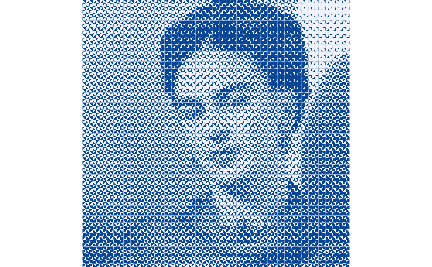
It is possible to randomize the tile allocation. A fascinating aspect of Truchet tiles is how the “texture” of the mosaic changes with each variation in the placement of tiles. For example:
# Set seed
seed <- 1085
set.seed(seed)

# Randomly select tiles
tiles <- sample(c("Al", "Bl", "Cl", "Dl"), size = 4, replace = TRUE)

value <- 3/4
# Design the mosaic
df <- frida_df %>%
  # Reverse the y axis
  mutate(y = -(y - max(y)),
         tiles = case_when(x %% 2 == 1 & y %% 2 == 0 ~ tiles[1],
                           x %% 2 == 0 & y %% 2 == 0 ~ tiles[2],
                           x %% 2 == 1 & y %% 2 == 1 ~ tiles[3],
                           x %% 2 == 0 & y %% 2 == 1 ~ tiles[4]),
         # Important! Notice the adjustment to the values to ensure that the area correctly reflects the underlying darkness value
         b = case_when(tiles == "Al" ~ 1- value,
                       tiles == "Bl" ~ 1- value,
                       tiles == "Cl" ~ value,
                       tiles == "Dl" ~ value))

# Assemble mosaic
mosaic <- st_truchet_fm(df = df %>% mutate(b = b * 0.99 + 0.001))

# Plot
mosaic %>%
  ggplot() +
  geom_sf(aes(fill = color),
          color = NA) +
  scale_fill_distiller(direction = 1) +
  coord_sf(expand = FALSE) +
  theme_void() +
  theme(legend.position = "none")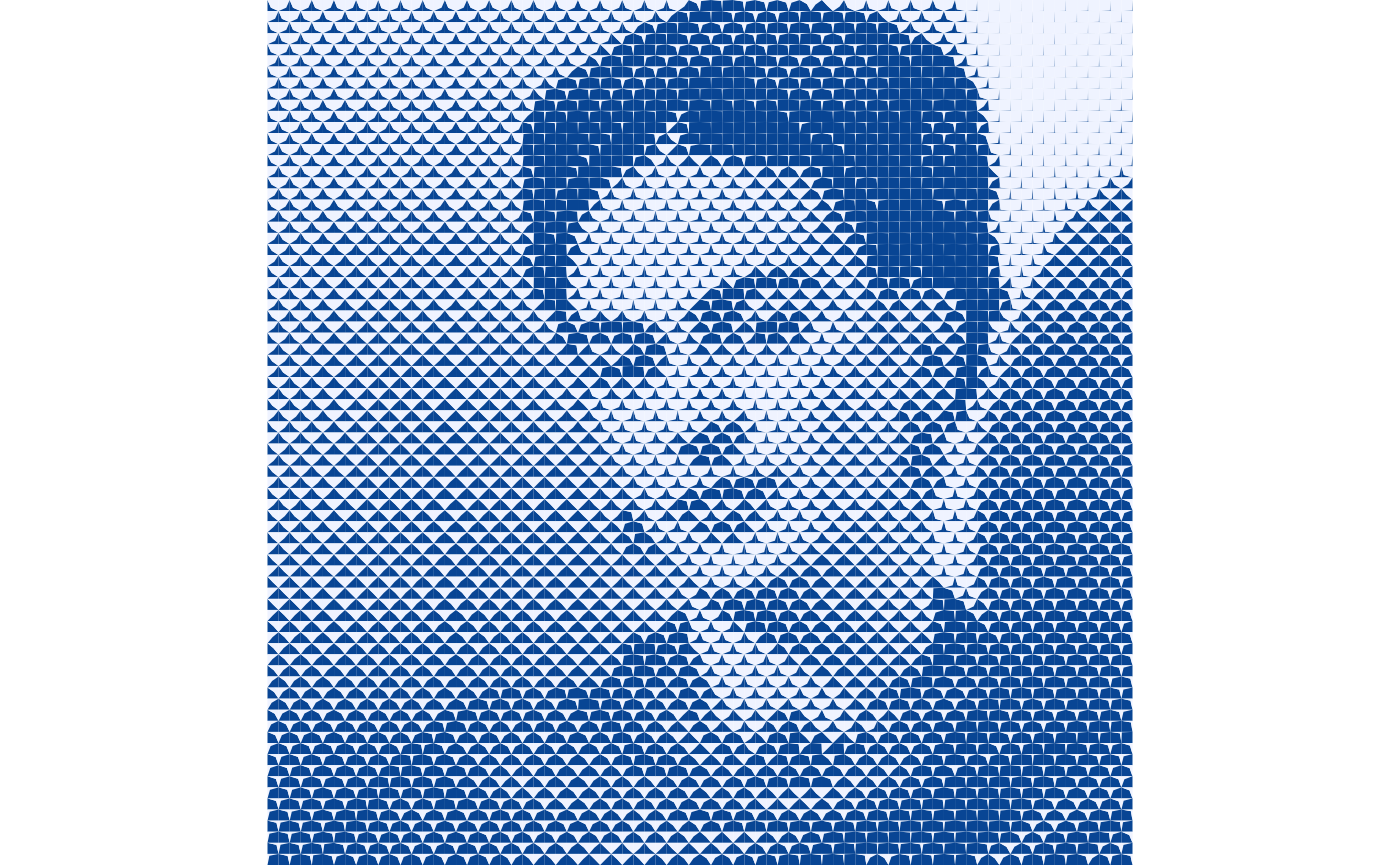
A nice feature of working with tiles as spatial data is that we can
perform geometric operations, such as st_nearest_feature()
from the {sf} package. The next example illustrate how to “borrow” the
colors of the underlying image.
Load the source image:
flower <- load.image(system.file("extdata",
                                 "flower.jpg",
                                 package = "truchet"))
The image is quite colorful:
plot(flower)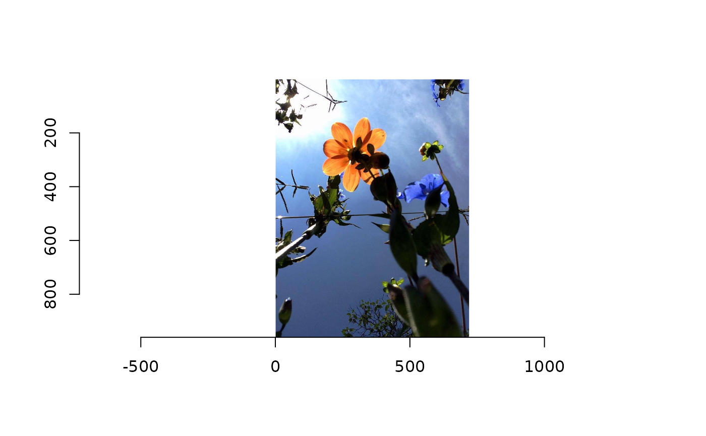
Resize image:
flower_rs <- imresize(flower, scale = 1/15, interpolation = 6)As before, we convert to grayscale and then to data frame:
flower_df <- flower_rs %>%
  grayscale() %>%
  as.data.frame()
This time, though, we also convert image to a data frame but retrieve the colors:
flower_color_df <- flower_rs %>%
  as.data.frame(wide="c") %>%
  # Reverse the y axis
  mutate(y = -(y - max(y)),
         hex_color = rgb(c.1,
                         c.2,
                         c.3))
Use Design C for the mosaic:
df <- flower_df %>%
  # Reverse the y axis
  mutate(y = -(y - max(y)),
         # The modulus of x + y can be used to create a checkerboard pattern
         tiles = case_when((x + y) %% 2 == 0 ~ "Al",
                           (x + y) %% 2 == 1 ~ "Cl"),
         b = case_when((x + y) %% 2 == 0 ~ 1 - value,
                       (x + y) %% 2 == 1 ~ value))

# Assemble the mosaic
mosaic <- st_truchet_fm(df = df %>% mutate(b = b * 0.80 + 0.001))
This is the duotone mosaic:
mosaic %>%
  ggplot() +
  geom_sf(aes(fill = color),
          color = NA) +
  scale_fill_distiller(direction = 1) +
  coord_sf(expand = FALSE) +
  theme_void() +
  theme(legend.position = "none")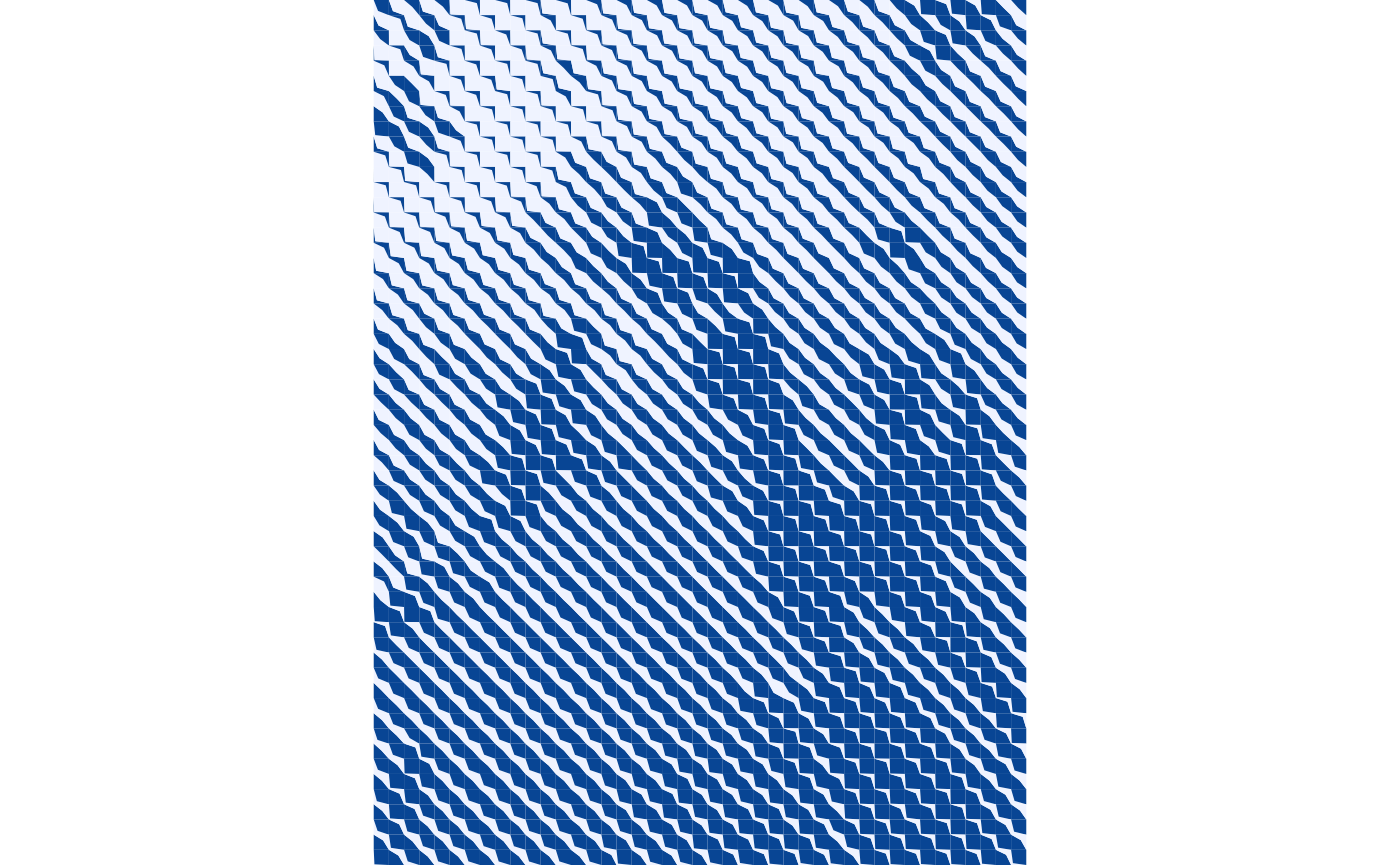
Convert the color data frame to simple features. This way we can use functions from the {sf} package to find the nearest feature to borrow the original colors in the image:
Find the nearest feature and borrow color:
hex_color <- flower_color_sf[mosaic %>%
                               st_nearest_feature(flower_color_sf),] %>%
  pull(hex_color)
We can now add the hexadecimal colors to the data frame with the mosaic:
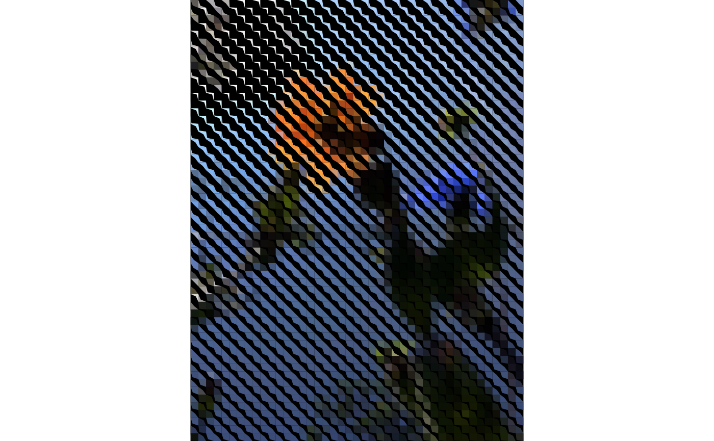
mosaic$hex_color <- hex_colorTo plot the mosaic we use the duotone colors to filter part of the tiles. For example, here we filter duotone color 2 and use the hexadecimal colors to fill the polygons:
mosaic %>%
  filter(color == 2) %>%
  ggplot() +
  geom_sf(aes(fill = hex_color),
          color = NA) +
  scale_fill_identity() +
  coord_sf(expand = FALSE) +
  theme_void() +
  theme(legend.position = "none")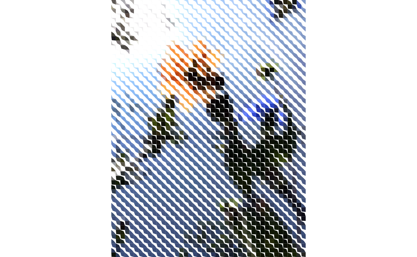
In this one, we filter the tiles with duotone color 1:
mosaic %>%
  filter(color == 1) %>%
  ggplot() +
  geom_sf(aes(fill = hex_color),
          color = NA) +
  scale_fill_identity() +
  coord_sf(expand = FALSE) +
  theme_void() +
  theme(legend.position = "none")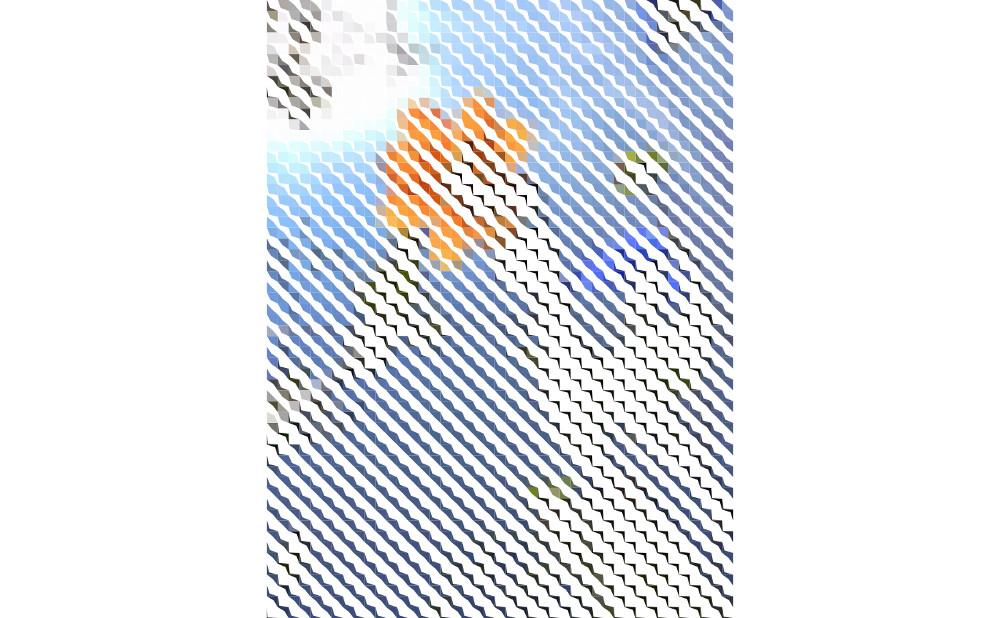
Playing with the background of the image can also lead to interesting results:
mosaic %>%
  filter(color == 2) %>%
  ggplot() +
  geom_sf(aes(fill = hex_color),
          color = NA) +
  scale_fill_identity() +
  coord_sf(expand = FALSE) +
  theme_void() +
  theme(panel.background = element_rect(fill = "black"),
        legend.position = "none")